9 Acquiescence Bias
Questionnaires usually assume that respondents select a response category because it best represents the content of the item. In practice, some people also differ in their tendency to agree with statements independently of what those statements say. This response style is called acquiescence (Cronbach, 1942; Robinson et al., 1991).
Acquiescence is therefore not simply “high responding” or extreme responding. It is a directional tendency toward endorsement that can operate across items with different substantive content.
This chapter develops acquiescence from three perspectives:
- What is acquiescence? — a response style with both stable and situational components.
- Why is it difficult to control? — reverse-keyed items can reveal acquiescence but can also introduce wording and comprehension effects.
- How can it be modeled? — factor-analytic response-bias models, random-intercept CFA, and random-intercept EGA.
The final section implements these approaches in R.
9.1 What Does Acquiescence Look Like?
Cronbach (1942) observed that respondents differed in how often they selected the affirmative response in true–false tests. The same logic extends to modern Likert-type questionnaires: an acquiescent respondent has a greater tendency to endorse statements regardless of their substantive polarity.
Consider a simplified Extraversion questionnaire:
| Item | Totally disagree | Partially disagree | Partially agree | Totally agree |
|---|---|---|---|---|
| I am a communicative person | 1 | 2 | 3 | 4 |
| I like interacting with people | 1 | 2 | 3 | 4 |
| I do not feel energized after large social interactions | 1 | 2 | 3 | 4 |
The important pattern is not that the respondent chooses extreme categories. The third response is substantively inconsistent with the first two after accounting for item polarity, yet the respondent still endorses the statement. This illustrates why balanced keying can provide information about acquiescence.
An extreme responder tends to choose endpoints such as 1 or 5. An acquiescent responder tends to choose the agreement side of the scale. A person can show one response style without showing the other.
9.2 Is Acquiescence a Trait or a State?
Acquiescence is associated with individual and contextual characteristics. Studies have reported relations with age, education, cognitive characteristics, and cultural context (Chen et al., 1995; Hinz et al., 2007; Soto et al., 2008). Twin research also suggests that acquiescence cannot be reduced to a simple inherited individual difference (Kam et al., 2013).
At the same time, some portion of acquiescence appears stable across measurement occasions (Billiet & Davidov, 2008). Latent state–trait analyses indicate that acquiescence contains both a relatively stable component and occasion-specific variation (Danner et al., 2015).
A useful interpretation is therefore:
| Component | Examples |
|---|---|
| Trait-like | Stable response habits, cognitive style, enduring person characteristics |
| State-like | Fatigue, motivation, interview context, momentary attention |
| Instrument-related | Item wording, response labels, balance of keyed directions |
This helps explain why acquiescence can generalize across content domains without necessarily being a psychological personality trait in the same sense as Extraversion or Neuroticism (Ferrando et al., 2004).
9.3 Why Acquiescence Matters
Even a modest acquiescence component can change the covariance structure of questionnaire data. Simulation and empirical studies show that it can distort factor recovery, affect regression or validity coefficients, and alter the apparent dimensionality of scales (Kam et al., 2012; Savalei & Falk, 2014; Valentini, 2017; Valentini & Hauck Filho, 2020).
One intuitive reason is that acquiescence creates shared variance among items that point in the same response direction. If this shared variance is not modeled, a factor analysis can interpret response-style covariance as substantive psychological covariance.
If acquiescence is expected to contribute meaningfully to the item covariance matrix, it should be considered before interpreting reliability, factor structure, or structural relations among latent variables (Billiet & McClendon, 2000; Cambré et al., 2002).
10 Reverse-Keyed Items: Solution and New Problem
A common strategy is to write some items in the positive direction of the construct and others in the opposite direction (Baumgartner & Steenkamp, 2001). For example:
- positive direction: “I often feel sad.”
- opposite direction: “I generally feel cheerful.”
After reverse scoring, both items are intended to point in the same substantive direction. If a respondent simply agrees with both, inconsistent substantive responses provide information about acquiescence.
This logic is useful, but reversing items is not psychometrically neutral.
10.1 1. Opposite wording may change cognitive processing
Negated and reverse-keyed items can require additional reading and interpretation. Respondents may misunderstand the negation, miss the key word, or use a different response process than they use for positively worded items (Van Sonderen et al., 2013; Weijters & Baumgartner, 2012).
These problems can be especially important when reading ability varies across respondents (Marsh, 1996).
10.2 2. Positive and negative items may not be substantively equivalent
Reversing wording assumes that the two item formulations represent opposite locations on one psychological continuum. That assumption is not always defensible (Chang, 1995; Suárez-Alvarez et al., 2018).
Agreeing with “I feel resilient” is not necessarily psychologically equivalent to disagreeing with “I give up easily.” The two statements may activate different content even if they are scored as opposites.
10.3 3. Reverse-keyed items can create method structure
Positive and reverse-keyed items sometimes form separate clusters or factors, particularly when a small subset of respondents answers the reverse-keyed items carelessly (Hughes, 2009; Knight et al., 1988; Woods, 2006).
Research has also found that scales containing only positively worded items can sometimes display cleaner covariance structures than mixed-key versions (Salazar, 2015; Schriesheim & Hill, 1981). This does not imply that acquiescence has disappeared; it may simply become harder to identify because all items share the same response direction.
If all items are positively keyed, acquiescence can contribute covariance in the same direction across the entire scale. A cleaner factor solution may therefore reflect less visible response-style conflict, not necessarily less response-style variance.
10.4 Should scales still contain oppositely keyed items?
There is no universal answer. The design involves a tradeoff:
| Potential advantage | Potential cost |
|---|---|
| Provides information for separating agreement tendency from content | Can introduce negation or wording-method effects |
| Helps identify random-intercept/acquiescence factors | Can increase respondent confusion |
| Makes uniform agreement patterns observable | Can create artificial positive-vs-negative item factors |
| Supports some balanced-scale methods | May be inappropriate when the construct has no natural opposite |
The key is to design substantively opposite items rather than simply adding grammatical negation whenever possible.
11 Statistical and Design-Based Control
Acquiescence can be addressed through both the measurement design and the statistical model.
11.1 Statistical control
Many models treat acquiescence as a latent response-style component that operates across items. This generally requires two substantive assumptions:
- the acquiescence component is distinguishable from the substantive latent traits; and
- the same response tendency contributes systematically across multiple items (Ferrando et al., 2003; Savalei & Falk, 2014).
Random-intercept item-factor models are a common example. Each item loads equally on a response-style factor, which captures a respondent’s general tendency to endorse higher or lower categories across the scale (Billiet & McClendon, 2000; Kam et al., 2012).
11.2 Questionnaire design
Scale format can also influence response styles. Research has examined response-category labeling, midpoint availability, keying direction, and alternative formats (Weijters et al., 2010).
Semantic differential scales are one alternative. In some applications, they show cleaner factor structure than agreement-style Likert items (Friborg et al., 2006). Another approach is the expanded format, where each response option is replaced by a substantive statement representing a different position on the construct (Zhang & Savalei, 2016).
A good statistical model cannot fully repair poorly written items, and good item writing cannot guarantee that response styles are absent. Response-process considerations should inform both the questionnaire design and the analysis.
12 Controlling Acquiescence in R
12.1 Approach 1: vampyr
The vampyr package implements the factor-analytic response-bias framework discussed in the previous chapter (Ferrando et al., 2009; Navarro-Gonzalez et al., 2021).
       V2              V8             V13             V21
 Min.   :1.000   Min.   :1.000   Min.   :1.000   Min.   :1.000
 1st Qu.:3.000   1st Qu.:2.000   1st Qu.:1.000   1st Qu.:2.000
 Median :4.000   Median :4.000   Median :2.000   Median :3.000
 Mean   :3.667   Mean   :3.263   Mean   :2.317   Mean   :2.947
 3rd Qu.:5.000   3rd Qu.:4.000   3rd Qu.:3.000   3rd Qu.:4.000
 Max.   :5.000   Max.   :5.000   Max.   :5.000   Max.   :5.000
       V1              V6             V17            V19             V20
 Min.   :1.000   Min.   :1.000   Min.   :1.00   Min.   :1.000   Min.   :1.000
 1st Qu.:3.000   1st Qu.:1.000   1st Qu.:3.00   1st Qu.:3.000   1st Qu.:1.000
 Median :4.000   Median :2.000   Median :4.00   Median :4.000   Median :2.000
 Mean   :3.643   Mean   :2.467   Mean   :3.71   Mean   :3.493   Mean   :1.997
 3rd Qu.:5.000   3rd Qu.:3.000   3rd Qu.:5.00   3rd Qu.:5.000   3rd Qu.:3.000
 Max.   :5.000   Max.   :5.000   Max.   :5.00   Max.   :5.000   Max.   :5.000
      V25
 Min.   :1.000
 1st Qu.:1.000
 Median :1.000
 Mean   :1.687
 3rd Qu.:2.000
 Max.   :5.000
The example dataset contains 300 respondents, four social-desirability markers, and six physical-aggression items with both positively and negatively keyed indicators.
DETAILS OF ANALYSIS

Number of participants                      :   300
Number of items                             :    10
Items selected as SD items                  :  1, 2, 3, 4
Dispersion Matrix                           : Polychoric Correlations
Method for factor extraction                : Unweighted Least Squares (ULS)
Rotation Method                             : none

-----------------------------------------------------------------------

Univariate item descriptives

Item       Mean        Variance    Skewness     Kurtosis (Zero centered)

Item   1   3.667       1.260      -0.555       -0.566
Item   2   3.263       1.760      -0.379       -1.005
Item   3   2.317       1.695       0.601       -0.880
Item   4   2.947       1.924      -0.033       -1.284
Item   5   3.643       1.374      -0.565       -0.535
Item   6   2.467       1.802       0.487       -0.967
Item   7   3.710       1.678      -0.652       -0.716
Item   8   3.493       1.629      -0.411       -0.862
Item   9   1.997       1.515       1.041       -0.011
Item  10   1.687       0.925       1.293        0.838

Polychoric correlation is advised when the univariate distributions of ordinal items are
asymmetric or with excess of kurtosis. If both indices are lower than one in absolute value,
then Pearson correlation is advised. You can read more about this subject in:

Muthen, B., & Kaplan D. (1985). A Comparison of Some Methodologies for the Factor Analysis of
Non-Normal Likert Variables. British Journal of Mathematical and Statistical Psychology, 38, 171-189.

Muthen, B., & Kaplan D. (1992). A Comparison of Some Methodologies for the Factor Analysis of
Non-Normal Likert Variables: A Note on the Size of the Model. British Journal of Mathematical
and Statistical Psychology, 45, 19-30.

-----------------------------------------------------------------------

Adequacy of the dispersion matrix

Determinant of the matrix     = 0.047816437916936
Bartlett's statistic          =   896.4 (df =    45; P = 0.000000)
Kaiser-Meyer-Olkin (KMO) test = 0.76664 (fair)

-----------------------------------------------------------------------
EXPLORATORY FACTOR ANALYSIS CONTROLLING SOCIAL DESIRABILITY AND ACQUIESCENCE
-----------------------------------------------------------------------

Robust Goodness of Fit statistics

          Root Mean Square Error of Approximation (RMSEA) = 0.032

 Robust Mean-Scaled Chi Square with 23 degrees of freedom = 30.146

              Non-Normed Fit Index (NNFI; Tucker & Lewis) = 0.989
                              Comparative Fit Index (CFI) = 0.994
                              Goodness of Fit Index (GFI) = 0.977

-----------------------------------------------------------------------

                  Root Mean Square Residuals (RMSR) = 0.0452
Expected mean value of RMSR for an acceptable model = 0.0578 (Kelley's criterion)

-----------------------------------------------------------------------

Unrotated loading matrix

         Factor SD Factor AC Factor 1
Item   1   0.60257   0.00000  0.00000
Item   2   0.51526   0.00000  0.00000
Item   3   0.72710   0.00000  0.00000
Item   4   0.71131   0.00000  0.00000
Item   5  -0.07851   0.23762 -0.54831
Item   6   0.27520   0.00235  0.49059
Item   7  -0.16412   0.57405 -0.70143
Item   8  -0.14320   0.54055 -0.59111
Item   9   0.26559   0.19617  0.66808
Item  10   0.31732   0.06252  0.68219
contAC = TRUE requests control for acquiescence. The SD_items argument additionally identifies the social-desirability markers. Therefore:
- to model both social desirability and acquiescence, retain both
SD_itemsandcontAC = TRUE; - to model acquiescence without a social-desirability marker factor, omit the
SD_itemsargument if permitted by the intended workflow; - to disable acquiescence control, use
contAC = FALSE.
If the item set is not balanced, the positions of items that do not have an opposite-key counterpart can be passed through unbalanced_items.
Factor scores can be requested by setting factor_scores = TRUE:
Computing EAP scores. Time remaining  0 seconds
Computing EAP scores. Time remaining  2 seconds
Computing EAP scores. Time remaining  1 seconds
Computing EAP scores. Time remaining  1 seconds
Computing EAP scores. Time remaining  2 seconds
Computing EAP scores. Time remaining  2 seconds
Computing EAP scores. Time remaining  2 seconds
Computing EAP scores. Time remaining  2 seconds
Computing EAP scores. Time remaining  2 seconds
Computing EAP scores. Time remaining  2 seconds
Computing EAP scores. Time remaining  2 seconds
Computing EAP scores. Time remaining  2 seconds
Computing EAP scores. Time remaining  2 seconds
Computing EAP scores. Time remaining  2 seconds
Computing EAP scores. Time remaining  2 seconds
Computing EAP scores. Time remaining  2 seconds
Computing EAP scores. Time remaining  2 seconds
Computing EAP scores. Time remaining  2 seconds
Computing EAP scores. Time remaining  2 seconds
Computing EAP scores. Time remaining  2 seconds
Computing EAP scores. Time remaining  2 seconds
Computing EAP scores. Time remaining  2 seconds
Computing EAP scores. Time remaining  2 seconds
Computing EAP scores. Time remaining  2 seconds
Computing EAP scores. Time remaining  2 seconds
Computing EAP scores. Time remaining  2 seconds
Computing EAP scores. Time remaining  2 seconds
Computing EAP scores. Time remaining  2 seconds
Computing EAP scores. Time remaining  2 seconds
Computing EAP scores. Time remaining  2 seconds
Computing EAP scores. Time remaining  2 seconds
Computing EAP scores. Time remaining  2 seconds
Computing EAP scores. Time remaining  2 seconds
Computing EAP scores. Time remaining  2 seconds
Computing EAP scores. Time remaining  2 seconds
Computing EAP scores. Time remaining  2 seconds
Computing EAP scores. Time remaining  2 seconds
Computing EAP scores. Time remaining  2 seconds
Computing EAP scores. Time remaining  2 seconds
Computing EAP scores. Time remaining  2 seconds
Computing EAP scores. Time remaining  2 seconds
Computing EAP scores. Time remaining  2 seconds
Computing EAP scores. Time remaining  2 seconds
Computing EAP scores. Time remaining  2 seconds
Computing EAP scores. Time remaining  2 seconds
Computing EAP scores. Time remaining  2 seconds
Computing EAP scores. Time remaining  2 seconds
Computing EAP scores. Time remaining  2 seconds
Computing EAP scores. Time remaining  2 seconds
Computing EAP scores. Time remaining  2 seconds
Computing EAP scores. Time remaining  2 seconds
Computing EAP scores. Time remaining  2 seconds
Computing EAP scores. Time remaining  2 seconds
Computing EAP scores. Time remaining  2 seconds
Computing EAP scores. Time remaining  2 seconds
Computing EAP scores. Time remaining  2 seconds
Computing EAP scores. Time remaining  2 seconds
Computing EAP scores. Time remaining  2 seconds
Computing EAP scores. Time remaining  2 seconds
Computing EAP scores. Time remaining  2 seconds
Computing EAP scores. Time remaining  2 seconds
Computing EAP scores. Time remaining  2 seconds
Computing EAP scores. Time remaining  2 seconds
Computing EAP scores. Time remaining  2 seconds
Computing EAP scores. Time remaining  2 seconds
Computing EAP scores. Time remaining  2 seconds
Computing EAP scores. Time remaining  2 seconds
Computing EAP scores. Time remaining  2 seconds
Computing EAP scores. Time remaining  2 seconds
Computing EAP scores. Time remaining  2 seconds
Computing EAP scores. Time remaining  2 seconds
Computing EAP scores. Time remaining  2 seconds
Computing EAP scores. Time remaining  2 seconds
Computing EAP scores. Time remaining  2 seconds
Computing EAP scores. Time remaining  2 seconds
Computing EAP scores. Time remaining  2 seconds
Computing EAP scores. Time remaining  2 seconds
Computing EAP scores. Time remaining  2 seconds
Computing EAP scores. Time remaining  2 seconds
Computing EAP scores. Time remaining  2 seconds
Computing EAP scores. Time remaining  2 seconds
Computing EAP scores. Time remaining  2 seconds
Computing EAP scores. Time remaining  2 seconds
Computing EAP scores. Time remaining  2 seconds
Computing EAP scores. Time remaining  2 seconds
Computing EAP scores. Time remaining  2 seconds
Computing EAP scores. Time remaining  2 seconds
Computing EAP scores. Time remaining  2 seconds
Computing EAP scores. Time remaining  2 seconds
Computing EAP scores. Time remaining  2 seconds
Computing EAP scores. Time remaining  2 seconds
Computing EAP scores. Time remaining  2 seconds
Computing EAP scores. Time remaining  2 seconds
Computing EAP scores. Time remaining  2 seconds
Computing EAP scores. Time remaining  2 seconds
Computing EAP scores. Time remaining  2 seconds
Computing EAP scores. Time remaining  2 seconds
Computing EAP scores. Time remaining  2 seconds
Computing EAP scores. Time remaining  2 seconds
Computing EAP scores. Time remaining  2 seconds
Computing EAP scores. Time remaining  2 seconds
Computing EAP scores. Time remaining  2 seconds
Computing EAP scores. Time remaining  2 seconds
Computing EAP scores. Time remaining  2 seconds
Computing EAP scores. Time remaining  2 seconds
Computing EAP scores. Time remaining  2 seconds
Computing EAP scores. Time remaining  2 seconds
Computing EAP scores. Time remaining  2 seconds
Computing EAP scores. Time remaining  2 seconds
Computing EAP scores. Time remaining  2 seconds
Computing EAP scores. Time remaining  2 seconds
Computing EAP scores. Time remaining  2 seconds
Computing EAP scores. Time remaining  2 seconds
Computing EAP scores. Time remaining  2 seconds
Computing EAP scores. Time remaining  2 seconds
Computing EAP scores. Time remaining  2 seconds
Computing EAP scores. Time remaining  2 seconds
Computing EAP scores. Time remaining  2 seconds
Computing EAP scores. Time remaining  2 seconds
Computing EAP scores. Time remaining  2 seconds
Computing EAP scores. Time remaining  2 seconds
Computing EAP scores. Time remaining  1 seconds
Computing EAP scores. Time remaining  2 seconds
Computing EAP scores. Time remaining  1 seconds
Computing EAP scores. Time remaining  1 seconds
Computing EAP scores. Time remaining  1 seconds
Computing EAP scores. Time remaining  1 seconds
Computing EAP scores. Time remaining  1 seconds
Computing EAP scores. Time remaining  1 seconds
Computing EAP scores. Time remaining  1 seconds
Computing EAP scores. Time remaining  1 seconds
Computing EAP scores. Time remaining  1 seconds
Computing EAP scores. Time remaining  1 seconds
Computing EAP scores. Time remaining  1 seconds
Computing EAP scores. Time remaining  1 seconds
Computing EAP scores. Time remaining  1 seconds
Computing EAP scores. Time remaining  1 seconds
Computing EAP scores. Time remaining  1 seconds
Computing EAP scores. Time remaining  1 seconds
Computing EAP scores. Time remaining  1 seconds
Computing EAP scores. Time remaining  1 seconds
Computing EAP scores. Time remaining  1 seconds
Computing EAP scores. Time remaining  1 seconds
Computing EAP scores. Time remaining  1 seconds
Computing EAP scores. Time remaining  1 seconds
Computing EAP scores. Time remaining  1 seconds
Computing EAP scores. Time remaining  1 seconds
Computing EAP scores. Time remaining  1 seconds
Computing EAP scores. Time remaining  1 seconds
Computing EAP scores. Time remaining  1 seconds
Computing EAP scores. Time remaining  1 seconds
Computing EAP scores. Time remaining  1 seconds
Computing EAP scores. Time remaining  1 seconds
Computing EAP scores. Time remaining  1 seconds
Computing EAP scores. Time remaining  1 seconds
Computing EAP scores. Time remaining  1 seconds
Computing EAP scores. Time remaining  1 seconds
Computing EAP scores. Time remaining  1 seconds
Computing EAP scores. Time remaining  1 seconds
Computing EAP scores. Time remaining  1 seconds
Computing EAP scores. Time remaining  1 seconds
Computing EAP scores. Time remaining  1 seconds
Computing EAP scores. Time remaining  1 seconds
Computing EAP scores. Time remaining  1 seconds
Computing EAP scores. Time remaining  1 seconds
Computing EAP scores. Time remaining  1 seconds
Computing EAP scores. Time remaining  1 seconds
Computing EAP scores. Time remaining  1 seconds
Computing EAP scores. Time remaining  1 seconds
Computing EAP scores. Time remaining  1 seconds
Computing EAP scores. Time remaining  1 seconds
Computing EAP scores. Time remaining  1 seconds
Computing EAP scores. Time remaining  1 seconds
Computing EAP scores. Time remaining  1 seconds
Computing EAP scores. Time remaining  1 seconds
Computing EAP scores. Time remaining  1 seconds
Computing EAP scores. Time remaining  1 seconds
Computing EAP scores. Time remaining  1 seconds
Computing EAP scores. Time remaining  1 seconds
Computing EAP scores. Time remaining  1 seconds
Computing EAP scores. Time remaining  1 seconds
Computing EAP scores. Time remaining  1 seconds
Computing EAP scores. Time remaining  1 seconds
Computing EAP scores. Time remaining  1 seconds
Computing EAP scores. Time remaining  1 seconds
Computing EAP scores. Time remaining  1 seconds
Computing EAP scores. Time remaining  1 seconds
Computing EAP scores. Time remaining  1 seconds
Computing EAP scores. Time remaining  1 seconds
Computing EAP scores. Time remaining  1 seconds
Computing EAP scores. Time remaining  1 seconds
Computing EAP scores. Time remaining  1 seconds
Computing EAP scores. Time remaining  1 seconds
Computing EAP scores. Time remaining  1 seconds
Computing EAP scores. Time remaining  1 seconds
Computing EAP scores. Time remaining  1 seconds
Computing EAP scores. Time remaining  1 seconds
Computing EAP scores. Time remaining  1 seconds
Computing EAP scores. Time remaining  1 seconds
Computing EAP scores. Time remaining  1 seconds
Computing EAP scores. Time remaining  1 seconds
Computing EAP scores. Time remaining  1 seconds
Computing EAP scores. Time remaining  1 seconds
Computing EAP scores. Time remaining  1 seconds
Computing EAP scores. Time remaining  1 seconds
Computing EAP scores. Time remaining  1 seconds
Computing EAP scores. Time remaining  1 seconds
Computing EAP scores. Time remaining  1 seconds
Computing EAP scores. Time remaining  1 seconds
Computing EAP scores. Time remaining  1 seconds
Computing EAP scores. Time remaining  1 seconds
Computing EAP scores. Time remaining  1 seconds
Computing EAP scores. Time remaining  1 seconds
Computing EAP scores. Time remaining  1 seconds
Computing EAP scores. Time remaining  1 seconds
Computing EAP scores. Time remaining  1 seconds
Computing EAP scores. Time remaining  1 seconds
Computing EAP scores. Time remaining  1 seconds
Computing EAP scores. Time remaining  1 seconds
Computing EAP scores. Time remaining  1 seconds
Computing EAP scores. Time remaining  1 seconds
Computing EAP scores. Time remaining  1 seconds
Computing EAP scores. Time remaining  1 seconds
Computing EAP scores. Time remaining  1 seconds
Computing EAP scores. Time remaining  1 seconds
Computing EAP scores. Time remaining  1 seconds
Computing EAP scores. Time remaining  1 seconds
Computing EAP scores. Time remaining  1 seconds
Computing EAP scores. Time remaining  1 seconds
Computing EAP scores. Time remaining  1 seconds
Computing EAP scores. Time remaining  1 seconds
Computing EAP scores. Time remaining  1 seconds
Computing EAP scores. Time remaining  1 seconds
Computing EAP scores. Time remaining  1 seconds
Computing EAP scores. Time remaining  1 seconds
Computing EAP scores. Time remaining  1 seconds
Computing EAP scores. Time remaining  1 seconds
Computing EAP scores. Time remaining  1 seconds
Computing EAP scores. Time remaining  1 seconds
Computing EAP scores. Time remaining  1 seconds
Computing EAP scores. Time remaining  1 seconds
Computing EAP scores. Time remaining  1 seconds
Computing EAP scores. Time remaining  1 seconds
Computing EAP scores. Time remaining  1 seconds
Computing EAP scores. Time remaining  1 seconds
Computing EAP scores. Time remaining  1 seconds
Computing EAP scores. Time remaining  1 seconds
Computing EAP scores. Time remaining  1 seconds
Computing EAP scores. Time remaining  1 seconds
Computing EAP scores. Time remaining  1 seconds
Computing EAP scores. Time remaining  1 seconds
Computing EAP scores. Time remaining  1 seconds
Computing EAP scores. Time remaining  1 seconds
Computing EAP scores. Time remaining  1 seconds
Computing EAP scores. Time remaining  1 seconds
Computing EAP scores. Time remaining  1 seconds
Computing EAP scores. Time remaining  1 seconds
Computing EAP scores. Time remaining  1 seconds
Computing EAP scores. Time remaining  1 seconds
Computing EAP scores. Time remaining  1 seconds
Computing EAP scores. Time remaining  1 seconds
Computing EAP scores. Time remaining  1 seconds
Computing EAP scores. Time remaining  1 seconds
Computing EAP scores. Time remaining  1 seconds
Computing EAP scores. Time remaining  1 seconds
Computing EAP scores. Time remaining  1 seconds
Computing EAP scores. Time remaining  1 seconds
Computing EAP scores. Time remaining  1 seconds
Computing EAP scores. Time remaining  1 seconds
Computing EAP scores. Time remaining  1 seconds
Computing EAP scores. Time remaining  1 seconds
Computing EAP scores. Time remaining  1 seconds
Computing EAP scores. Time remaining  1 seconds
Computing EAP scores. Time remaining  1 seconds
Computing EAP scores. Time remaining  1 seconds
Computing EAP scores. Time remaining  1 seconds
Computing EAP scores. Time remaining  1 seconds
Computing EAP scores. Time remaining  1 seconds
Computing EAP scores. Time remaining  1 seconds
Computing EAP scores. Time remaining  1 seconds
Computing EAP scores. Time remaining  1 seconds
Computing EAP scores. Time remaining  1 seconds
Computing EAP scores. Time remaining  1 seconds
Computing EAP scores. Time remaining  1 seconds
Computing EAP scores. Time remaining  1 seconds
Computing EAP scores. Time remaining  1 seconds
Computing EAP scores. Time remaining  1 seconds
Computing EAP scores. Time remaining  1 seconds
Computing EAP scores. Time remaining  1 seconds
Computing EAP scores. Time remaining  1 seconds
Computing EAP scores. Time remaining  1 seconds
Computing EAP scores. Time remaining  1 seconds
Computing EAP scores. Time remaining  1 seconds
Computing EAP scores. Time remaining  1 seconds
Computing EAP scores. Time remaining  1 seconds
Computing EAP scores. Time remaining  1 seconds
Computing EAP scores. Time remaining  1 seconds
Computing EAP scores. Time remaining  1 seconds
Computing EAP scores. Time remaining  1 seconds
Computing EAP scores. Time remaining  0 seconds


DETAILS OF ANALYSIS

Number of participants                      :   300
Number of items                             :    10
Items selected as SD items                  :  1, 2, 3, 4
Dispersion Matrix                           : Polychoric Correlations
Method for factor extraction                : Unweighted Least Squares (ULS)
Rotation Method                             : none

-----------------------------------------------------------------------

Univariate item descriptives

Item       Mean        Variance    Skewness     Kurtosis (Zero centered)

Item   1   3.667       1.260      -0.555       -0.566
Item   2   3.263       1.760      -0.379       -1.005
Item   3   2.317       1.695       0.601       -0.880
Item   4   2.947       1.924      -0.033       -1.284
Item   5   3.643       1.374      -0.565       -0.535
Item   6   2.467       1.802       0.487       -0.967
Item   7   3.710       1.678      -0.652       -0.716
Item   8   3.493       1.629      -0.411       -0.862
Item   9   1.997       1.515       1.041       -0.011
Item  10   1.687       0.925       1.293        0.838

Polychoric correlation is advised when the univariate distributions of ordinal items are
asymmetric or with excess of kurtosis. If both indices are lower than one in absolute value,
then Pearson correlation is advised. You can read more about this subject in:

Muthen, B., & Kaplan D. (1985). A Comparison of Some Methodologies for the Factor Analysis of
Non-Normal Likert Variables. British Journal of Mathematical and Statistical Psychology, 38, 171-189.

Muthen, B., & Kaplan D. (1992). A Comparison of Some Methodologies for the Factor Analysis of
Non-Normal Likert Variables: A Note on the Size of the Model. British Journal of Mathematical
and Statistical Psychology, 45, 19-30.

-----------------------------------------------------------------------

Adequacy of the dispersion matrix

Determinant of the matrix     = 0.047816437916936
Bartlett's statistic          =   896.4 (df =    45; P = 0.000000)
Kaiser-Meyer-Olkin (KMO) test = 0.76664 (fair)

-----------------------------------------------------------------------
EXPLORATORY FACTOR ANALYSIS CONTROLLING SOCIAL DESIRABILITY AND ACQUIESCENCE
-----------------------------------------------------------------------

Robust Goodness of Fit statistics

          Root Mean Square Error of Approximation (RMSEA) = 0.032

 Robust Mean-Scaled Chi Square with 23 degrees of freedom = 30.146

              Non-Normed Fit Index (NNFI; Tucker & Lewis) = 0.989
                              Comparative Fit Index (CFI) = 0.994
                              Goodness of Fit Index (GFI) = 0.977

-----------------------------------------------------------------------

                  Root Mean Square Residuals (RMSR) = 0.0452
Expected mean value of RMSR for an acceptable model = 0.0578 (Kelley's criterion)

-----------------------------------------------------------------------

Unrotated loading matrix

         Factor SD Factor AC Factor 1
Item   1   0.60253   0.00000  0.00000
Item   2   0.51526   0.00000  0.00000
Item   3   0.72704   0.00000  0.00000
Item   4   0.71131   0.00000  0.00000
Item   5  -0.07850   0.23753  0.54832
Item   6   0.27518   0.00260 -0.49070
Item   7  -0.16411   0.57389  0.70153
Item   8  -0.14319   0.54036  0.59123
Item   9   0.26558   0.19654 -0.66825
Item  10   0.31730   0.06258 -0.68213

-----------------------------------------------------------------------

RELIABILITY OF EAP SCORES

Factor         EAP Reliability estimate

SD           :  0.6740
Acquiescence :  0.4113
Factor 1     :  0.6594

PARTICIPANTS'S SCORES ON FACTORS:
Rescaled to mean = 50 and standard deviation = 10 in the sample

       Factor SD Factor AC Factor 1
  [1,]  44.30693  48.53333 51.44554
  [2,]  59.62589  38.14346 50.57165
  [3,]  61.19054  42.28909 57.66120
  [4,]  55.02773  43.35121 56.66889
  [5,]  48.23123  38.65266 39.70465
  [6,]  44.51619  64.27199 54.13617
  [7,]  44.73218  65.06108 43.76337
  [8,]  39.62591  50.47004 27.99325
  [9,]  61.35089  36.07724 54.53989
 [10,]  52.16276  54.34207 45.29344
 [11,]  55.76837  44.66200 43.94625
 [12,]  53.40863  58.25979 41.60500
 [13,]  46.66442  51.23092 48.62351
 [14,]  78.49640  78.23464 44.76011
 [15,]  55.73234  54.95433 44.28975
 [16,]  44.79371  64.49245 62.46085
 [17,]  45.01493  46.09226 43.67809
 [18,]  44.88499  59.50155 44.67008
 [19,]  43.98230  35.50952 32.96192
 [20,]  56.02719  34.92454 45.45263
 [21,]  43.26996  33.50331 56.80886
 [22,]  55.84810  64.01859 33.23316
 [23,]  28.11587  58.09739 66.63817
 [24,]  49.33801  42.43831 49.35854
 [25,]  39.88321  45.29596 52.73939
 [26,]  37.03512  57.52852 57.22556
 [27,]  55.01006  47.35659 52.52035
 [28,]  55.91189  62.54358 49.19137
 [29,]  43.96927  45.20916 43.43612
 [30,]  55.62030  44.38434 44.27717
 [31,]  37.85433  65.94432 58.47460
 [32,]  44.88425  43.32807 54.77204
 [33,]  46.71557  40.36808 37.19440
 [34,]  65.13345  49.63985 50.15156
 [35,]  47.81356  48.87639 49.12380
 [36,]  67.06698  41.07036 59.82670
 [37,]  44.91543  53.52469 46.46942
 [38,]  54.26559  57.86662 32.03135
 [39,]  55.62404  44.10899 43.98672
 [40,]  43.18532  54.51220 43.88604
 [41,]  52.53533  46.38576 41.35634
 [42,]  64.91994  50.81471 51.36486
 [43,]  65.34059  53.50234 57.04835
 [44,]  54.85163  42.89256 45.58115
 [45,]  55.73981  55.70850 44.26563
 [46,]  52.50882  44.32568 44.69953
 [47,]  34.77887  41.68987 47.26047
 [48,]  45.26524  45.00766 43.73164
 [49,]  32.23291  36.27044 49.27663
 [50,]  55.73959  43.90253 55.99082
 [51,]  32.22156  56.28429 43.71595
 [52,]  49.72514  51.33507 58.72944
 [53,]  46.29025  38.95594 48.76390
 [54,]  50.73533  58.75385 69.74790
 [55,]  56.36102  50.67899 32.93594
 [56,]  34.49192  41.64343 61.91512
 [57,]  44.14591  50.13327 54.24789
 [58,]  44.05135  53.41648 46.56807
 [59,]  78.32611  61.80584 54.36919
 [60,]  46.94619  53.90221 45.60982
 [61,]  78.53930  71.25219 56.53518
 [62,]  55.64357  47.46930 44.28069
 [63,]  43.98645  53.49732 44.31058
 [64,]  57.69061  47.71755 35.95774
 [65,]  55.68321  42.59590 46.20676
 [66,]  55.60401  43.40642 44.26971
 [67,]  55.75838  56.92367 43.60277
 [68,]  64.71961  52.13575 43.68025
 [69,]  45.40345  60.14602 66.26557
 [70,]  48.54799  62.54567 62.93461
 [71,]  43.40130  44.68513 54.75671
 [72,]  43.79504  58.59898 68.77227
 [73,]  37.82186  58.41796 67.94224
 [74,]  72.69024  68.24316 59.96968
 [75,]  38.54384  60.71244 53.83940
 [76,]  44.39554  77.52443 33.66295
 [77,]  34.98427  43.00733 33.98936
 [78,]  42.29033  37.15494 52.27701
 [79,]  55.43507  33.83137 35.09011
 [80,]  41.18887  67.26499 56.56664
 [81,]  44.31976  50.68758 44.59956
 [82,]  78.46775  61.64153 69.53114
 [83,]  53.24704  71.48802 27.67509
 [84,]  41.16995  50.34212 56.71693
 [85,]  55.38692  62.01918 38.04596
 [86,]  44.96077  74.37443 21.44334
 [87,]  54.44571  39.64716 32.48738
 [88,]  51.48805  52.15982 54.15668
 [89,]  45.36171  43.59959 40.06175
 [90,]  55.82176  45.90922 54.09556
 [91,]  37.66055  71.91785 51.35576
 [92,]  44.12155  53.92820 46.05766
 [93,]  34.84139  66.23853 38.44514
 [94,]  54.82210  53.86959 45.82189
 [95,]  66.64004  51.15018 60.31911
 [96,]  67.81468  78.46926 44.26293
 [97,]  56.12442  51.66110 44.52901
 [98,]  33.52131  58.28471 67.34880
 [99,]  48.00178  51.28965 55.13201
[100,]  54.35116  53.20460 43.29480
[101,]  44.91259  68.10615 55.67961
[102,]  66.49296  44.37002 43.99023
[103,]  49.86741  66.59882 49.96871
[104,]  44.95405  65.13864 32.76418
[105,]  33.06061  48.67840 49.85371
[106,]  75.49319  42.91926 53.95907
[107,]  56.44580  55.56875 34.04476
[108,]  70.56629  54.84289 46.26655
[109,]  56.47430  66.37101 52.40816
[110,]  54.42747  50.12035 40.50429
[111,]  44.33562  46.81305 53.41868
[112,]  55.87860  50.70268 49.30562
[113,]  40.23125  46.74339 53.50564
[114,]  60.99905  46.10467 55.92798
[115,]  55.65068  34.94991 45.25854
[116,]  66.93604  44.63417 56.36218
[117,]  55.99772  56.97442 42.33407
[118,]  55.54234  58.38975 41.49610
[119,]  44.58544  49.90701 50.06975
[120,]  75.70712  57.31583 66.39735
[121,]  53.27660  48.42651 51.57274
[122,]  46.07506  37.19541 44.31314
[123,]  67.24756  55.06597 44.71137
[124,]  38.76309  50.00996 44.56689
[125,]  64.49795  52.48493 47.50387
[126,]  41.72542  58.53579 68.48474
[127,]  43.12616  46.42547 21.98973
[128,]  41.30243  45.13707 32.88256
[129,]  42.51628  62.30525 56.25193
[130,]  31.75905  35.57259 52.85979
[131,]  37.35715  75.96149 33.55345
[132,]  46.13451  58.64768 69.10241
[133,]  43.81907  41.37528 47.29721
[134,]  66.99948  55.75837 43.00825
[135,]  44.32081  36.68745 32.89073
[136,]  42.22120  58.55133 68.55349
[137,]  43.89334  48.57296 51.26597
[138,]  65.19329  49.36649 62.12677
[139,]  42.66200  71.27133 43.43428
[140,]  33.85796  58.29630 67.39340
[141,]  42.68680  46.67931 63.53368
[142,]  44.93812  52.99551 57.75789
[143,]  55.74570  46.77641 44.82189
[144,]  49.66252  58.72872 69.59873
[145,]  32.17716  47.61180 43.31868
[146,]  47.70755  40.15131 59.87204
[147,]  29.64881  58.01817 54.69417
[148,]  33.28783  40.07510 46.30938
[149,]  55.81802  46.33249 42.35236
[150,]  48.65142  58.70883 69.45463
[151,]  47.96954  55.06233 43.82333
[152,]  43.65859  38.22523 38.05658
[153,]  54.17576  46.08657 42.22037
[154,]  61.57690  49.03793 62.95040
[155,]  43.32867  58.58478 68.70746
[156,]  55.71130  58.85820 70.45301
[157,]  53.68410  55.24076 44.77955
[158,]  44.74147  57.75218 58.49819
[159,]  55.04700  47.04627 49.42422
[160,]  44.80917  58.62540 68.91409
[161,]  55.75041  63.31818 56.49360
[162,]  60.59537  46.32220 54.69732
[163,]  68.80053  42.99100 57.15267
[164,]  56.44475  64.90036 35.18837
[165,]  43.77049  43.79944 57.75513
[166,]  55.74922  52.55974 44.48193
[167,]  55.72438  45.39851 44.36239
[168,]  55.67117  49.90305 48.65478
[169,]  56.73583  68.12086 57.22961
[170,]  68.26663  40.70238 53.44398
[171,]  62.50599  67.14426 60.03550
[172,]  53.84318  47.51506 51.77765
[173,]  67.01732  55.69438 44.41920
[174,]  42.47457  57.65714 58.39502
[175,]  67.06228  47.50713 44.30888
[176,]  50.88671  63.05566 47.41429
[177,]  46.05298  60.55398 55.56958
[178,]  54.32736  55.21106 55.86801
[179,]  56.59291  46.34890 55.89768
[180,]  44.87827  49.55050 61.39963
[181,]  58.32160  44.61133 55.67777
[182,]  54.62206  47.86318 51.29531
[183,]  60.13668  58.59063 44.30436
[184,]  34.34853  58.31159 67.46095
[185,]  47.20400  58.67753 69.25098
[186,]  60.62814  46.21580 65.73782
[187,]  78.42786  58.69172 65.24703
[188,]  37.86733  57.55291 57.35776
[189,]  55.41221  42.20911 45.18345
[190,]  47.64655  54.34091 35.66668
[191,]  55.69738  44.73492 55.27301
[192,]  62.74181  44.59657 53.30229
[193,]  40.99746  49.14638 60.60332
[194,]  56.91781  47.76767 23.83859
[195,]  41.66001  40.42141 31.09670
[196,]  55.68602  39.82666 44.87841
[197,]  68.74878  61.65220 44.16419
[198,]  55.57637  56.17315 55.18519
[199,]  55.71428  69.80068 58.16348
[200,]  44.21216  56.42316 43.54466
[201,]  55.18579  47.83881 43.23304
[202,]  44.77232  69.69548 53.72343
[203,]  51.10243  41.47817 52.24413
[204,]  56.46084  77.80894 44.34424
[205,]  39.54510  60.63639 54.09999
[206,]  44.14082  60.15513 66.02529
[207,]  61.72457  43.40962 44.31042
[208,]  54.37954  46.29849 33.90631
[209,]  50.24051  46.51842 53.44186
[210,]  44.67903  48.55167 56.27340
[211,]  58.58784  57.01544 34.89663
[212,]  55.73781  58.86172 70.45222
[213,]  54.03654  32.77720 46.52539
[214,]  55.87161  58.86217 70.47479
[215,]  41.35863  50.65896 49.76773
[216,]  47.11890  52.41924 25.46364
[217,]  50.97341  67.98192 57.65033
[218,]  55.74759  51.40449 57.71154
[219,]  58.51399  43.21493 32.87924
[220,]  51.73471  42.11551 54.14053
[221,]  77.03195  50.62836 20.87354
[222,]  55.68614  66.10544 55.31267
[223,]  45.47022  48.19087 51.84919
[224,]  29.00478  62.70793 52.91521
[225,]  67.09957  44.87906 55.32408
[226,]  44.36715  66.30755 32.77596
[227,]  39.95301  36.14798 41.45555
[228,]  56.17832  36.70424 55.84522
[229,]  45.74690  60.14354 66.33147
[230,]  67.13419  46.00870 54.04177
[231,]  44.94682  55.42967 44.43491
[232,]  55.60031  44.88354 55.04719
[233,]  55.71751  43.85485 44.28774
[234,]  67.10088  44.62123 55.41465
[235,]  67.23702  35.23461 53.41365
[236,]  48.48319  58.70514 69.43099
[237,]  55.69196  44.54694 55.46071
[238,]  43.46558  45.45591 63.94042
[239,]  43.86880  33.04691 55.88409
[240,]  66.99831  44.58163 55.47372
[241,]  56.14206  44.02883 44.84155
[242,]  61.02549  38.22987 54.37303
[243,]  42.84727  51.91398 35.71997
[244,]  55.70342  59.35807 52.03293
[245,]  55.73563  55.37076 55.97727
[246,]  58.90692  58.03032 62.31620
[247,]  55.73359  44.57381 43.58576
[248,]  44.26833  38.82980 47.31009
[249,]  36.53438  75.32455 48.18661
[250,]  78.49796  54.79313 55.80569
[251,]  65.86789  45.78176 24.04964
[252,]  55.80809  44.30993 44.76013
[253,]  71.62196  44.53799 67.72502
[254,]  70.38684  51.52423 46.95256
[255,]  66.84969  36.94340 32.94678
[256,]  66.65261  60.64741 50.32906
[257,]  45.58429  45.56195 64.33035
[258,]  55.70542  47.15318 49.67167
[259,]  48.96152  51.76851 47.60459
[260,]  75.67421  46.47265 53.94876
[261,]  45.70155  46.84392 64.07378
[262,]  51.98984  43.83698 56.16502
[263,]  55.51901  71.16579 56.05550
[264,]  34.67720  29.95117 53.80839
[265,]  44.45824  67.55811 56.35699
[266,]  41.74108  58.53668 68.48679
[267,]  33.97296  58.63711 55.37404
[268,]  50.61076  58.92899 48.50386
[269,]  35.30877  63.29761 60.27346
[270,]  34.33379  34.60294 31.01479
[271,]  53.10675  42.90331 54.11253
[272,]  67.41024  45.39661 44.23895
[273,]  53.08258  60.09076 67.70576
[274,]  55.68563  72.88740 45.77337
[275,]  55.47507  57.59952 53.76175
[276,]  45.34361  58.63728 68.98923
[277,]  36.99583  70.18279 44.38520
[278,]  40.28448  53.76930 44.62264
[279,]  44.44515  56.11669 32.63906
[280,]  45.25829  59.73503 49.26898
[281,]  55.31328  60.07462 68.12385
[282,]  44.27962  62.84108 61.71772
[283,]  55.54118  47.68386 33.87229
[284,]  55.28901  38.82994 42.58729
[285,]  51.51234  58.77026 69.85777
[286,]  43.30875  57.65718 58.54995
[287,]  67.66592  69.67636 43.87207
[288,]  54.75927  65.90884 53.41881
[289,]  46.98778  37.41784 50.10966
[290,]  55.54860  44.00472 44.43358
[291,]  45.58042  46.66428 44.76454
[292,]  62.80568  55.74188 56.24008
[293,]  45.74401  51.35739 48.56243
[294,]  52.38182  44.70606 65.27921
[295,]  57.57962  50.80088 47.36610
[296,]  75.39490  65.89827 62.33904
[297,]  67.16584  45.44543 44.00016
[298,]  58.57901  36.36588 53.30822
[299,]  55.86654  42.66499 55.50919
[300,]  73.41983  45.74091 42.92351

NOTE: The precision matrices for the  3 factors were not printed for preventing console spacing issues.
These matrices are stored in $Precision_matrix in the output variable.As in the social-desirability chapter, these scores are model-dependent estimates rather than directly observed traits.
12.2 Approach 2: Random-Intercept CFA
A random-intercept item-factor model represents acquiescence as a common factor with equal loadings across items (Billiet & McClendon, 2000; Savalei & Falk, 2014). The substantive factors capture content, while the random-intercept factor captures a person’s general tendency to use higher or lower response categories.
We use lavaan (Rosseel, 2012) and the wmt2 dataset distributed with EGAnet (Golino & Christensen, 2023).
This is lavaan 0.7-2
lavaan is FREE software! Please report any bugs.[1;m[4;m
EGAnet (version 2.4.1)[0m[0m
For help getting started, see <https://r-ega.net>
For bugs and errors, submit an issue to <https://github.com/hfgolino/EGAnet/issues>12.2.1 Specify the model
Show random-intercept CFA syntax
model_RI <- '
              factor1 =~ NA*wmt1 + wmt2 + wmt3 + wmt5 + wmt11 +
              wmt12 + wmt13 + wmt15 + wmt16 + wmt17 + wmt18

              factor2 =~ NA*wmt4 + wmt6 + wmt7 + wmt8 +
              wmt9 + wmt10 + wmt14

              # Random Intercepts
              acquiescence =~ 1*wmt1 + 1*wmt2 + 1*wmt3 + 1*wmt5 +
              1*wmt11 + 1*wmt12 + 1*wmt13 + 1*wmt15 + 1*wmt16 +
              1*wmt17 + 1*wmt18 + 1*wmt4 + 1*wmt6 + 1*wmt7 +
              1*wmt8 + 1*wmt9 + 1*wmt10 + 1*wmt14

              factor1 ~~ 0*acquiescence
              factor2 ~~ 0*acquiescence

              acquiescence ~~ acquiescence

              factor1 ~~ 1*factor1
              factor2 ~~ 1*factor2
              '
The important part is:
Every indicator has a loading fixed to 1 on the acquiescence factor. This factor therefore represents a common person-specific response tendency rather than a content factor defined by differential item loadings.
The substantive factors are constrained to be orthogonal to the acquiescence factor. That is a strong but useful identification and interpretation assumption; it should be justified rather than treated as a purely technical detail.
12.2.2 Fit the ordinal CFA
lavaan 0.7-2 ended normally after 43 iterations

  Estimator                                       DWLS
  Optimization method                           NLMINB
  Number of model parameters                        38

  Number of observations                          1185

Model Test User Model:
                                              Standard      Scaled
  Test Statistic                               232.896     285.231
  Degrees of freedom                               133         133
  P-value (Unknown)                                 NA       0.000
  Scaling correction factor                                  0.873
  Shift parameter                                           18.557
    simple second-order correction

Model Test Baseline Model:

  Test statistic                             12385.490    7849.254
  Degrees of freedom                               153         153
  P-value                                           NA       0.000
  Scaling correction factor                                  1.589

User Model versus Baseline Model:

  Comparative Fit Index (CFI)                    0.992       0.980
  Tucker-Lewis Index (TLI)                       0.991       0.977

  Robust Comparative Fit Index (CFI)                         0.922
  Robust Tucker-Lewis Index (TLI)                            0.910

Root Mean Square Error of Approximation:

  RMSEA                                          0.025       0.031
  90 Percent confidence interval - lower         0.020       0.026
  90 Percent confidence interval - upper         0.030       0.036
  P-value H_0: RMSEA <= 0.050                    1.000       1.000
  P-value H_0: RMSEA >= 0.080                    0.000       0.000

  Robust RMSEA                                               0.065
  90 Percent confidence interval - lower                     0.054
  90 Percent confidence interval - upper                     0.076
  P-value H_0: Robust RMSEA <= 0.050                         0.011
  P-value H_0: Robust RMSEA >= 0.080                         0.012

Standardized Root Mean Square Residual:

  SRMR                                           0.052       0.052

Goodness of Fit Index:

  Goodness of Fit Index (GFI)                    0.991
  90 Percent confidence interval - lower         0.986
  90 Percent confidence interval - upper         0.994

  Robust GFI                                                 0.941
  90 Percent confidence interval - lower                     0.921
  90 Percent confidence interval - upper                     0.958

Parameter Estimates:

  Parameterization                               Delta
  Standard errors                           Robust.sem
  Information                                 Expected
  Information saturated (h1) model        Unstructured

Latent Variables:
                   Estimate  Std.Err  z-value  P(>|z|)   Std.lv  Std.all
  factor1 =~
    wmt1              0.233    0.065    3.580    0.000    0.233    0.233
    wmt2              0.607    0.066    9.213    0.000    0.607    0.607
    wmt3              0.449    0.061    7.410    0.000    0.449    0.449
    wmt5              0.314    0.062    5.054    0.000    0.314    0.314
    wmt11             0.019    0.074    0.260    0.795    0.019    0.019
    wmt12             0.061    0.074    0.828    0.408    0.061    0.061
    wmt13             0.110    0.069    1.603    0.109    0.110    0.110
    wmt15             0.136    0.070    1.947    0.052    0.136    0.136
    wmt16             0.126    0.071    1.772    0.076    0.126    0.126
    wmt17            -0.044    0.078   -0.568    0.570   -0.044   -0.044
    wmt18            -0.339    0.098   -3.452    0.001   -0.339   -0.339
  factor2 =~
    wmt4              0.300    0.056    5.328    0.000    0.300    0.300
    wmt6              0.504    0.052    9.750    0.000    0.504    0.504
    wmt7              0.352    0.055    6.452    0.000    0.352    0.352
    wmt8              0.269    0.057    4.695    0.000    0.269    0.269
    wmt9              0.393    0.054    7.292    0.000    0.393    0.393
    wmt10             0.477    0.054    8.910    0.000    0.477    0.477
    wmt14             0.227    0.060    3.817    0.000    0.227    0.227
  acquiescence =~
    wmt1              1.000                               0.580    0.580
    wmt2              1.000                               0.580    0.580
    wmt3              1.000                               0.580    0.580
    wmt5              1.000                               0.580    0.580
    wmt11             1.000                               0.580    0.580
    wmt12             1.000                               0.580    0.580
    wmt13             1.000                               0.580    0.580
    wmt15             1.000                               0.580    0.580
    wmt16             1.000                               0.580    0.580
    wmt17             1.000                               0.580    0.580
    wmt18             1.000                               0.580    0.580
    wmt4              1.000                               0.580    0.580
    wmt6              1.000                               0.580    0.580
    wmt7              1.000                               0.580    0.580
    wmt8              1.000                               0.580    0.580
    wmt9              1.000                               0.580    0.580
    wmt10             1.000                               0.580    0.580
    wmt14             1.000                               0.580    0.580

Covariances:
                   Estimate  Std.Err  z-value  P(>|z|)   Std.lv  Std.all
  factor1 ~~
    acquiescence      0.000                               0.000    0.000
  factor2 ~~
    acquiescence      0.000                               0.000    0.000
  factor1 ~~
    factor2           0.591    0.078    7.602    0.000    0.591    0.591

Thresholds:
                   Estimate  Std.Err  z-value  P(>|z|)   Std.lv  Std.all
    wmt1|t1          -0.475    0.038  -12.521    0.000   -0.475   -0.475
    wmt2|t1          -0.881    0.042  -20.956    0.000   -0.881   -0.881
    wmt3|t1          -0.651    0.039  -16.544    0.000   -0.651   -0.651
    wmt5|t1          -0.475    0.038  -12.521    0.000   -0.475   -0.475
    wmt11|t1          0.447    0.038   11.833    0.000    0.447    0.447
    wmt12|t1          0.471    0.038   12.406    0.000    0.471    0.471
    wmt13|t1          0.195    0.037    5.311    0.000    0.195    0.195
    wmt15|t1          0.445    0.038   11.776    0.000    0.445    0.445
    wmt16|t1          0.412    0.038   10.972    0.000    0.412    0.412
    wmt17|t1          0.815    0.041   19.787    0.000    0.815    0.815
    wmt18|t1          0.641    0.039   16.320    0.000    0.641    0.641
    wmt4|t1          -0.158    0.037   -4.325    0.000   -0.158   -0.158
    wmt6|t1          -0.355    0.037   -9.533    0.000   -0.355   -0.355
    wmt7|t1          -0.208    0.037   -5.658    0.000   -0.208   -0.208
    wmt8|t1           0.116    0.037    3.164    0.002    0.116    0.116
    wmt9|t1          -0.158    0.037   -4.325    0.000   -0.158   -0.158
    wmt10|t1         -0.280    0.037   -7.569    0.000   -0.280   -0.280
    wmt14|t1          0.128    0.037    3.513    0.000    0.128    0.128

Variances:
                   Estimate  Std.Err  z-value  P(>|z|)   Std.lv  Std.all
    acquiescence      0.337    0.016   21.029    0.000    1.000    1.000
    factor1           1.000                               1.000    1.000
    factor2           1.000                               1.000    1.000
   .wmt1              0.609                               0.609    0.609
   .wmt2              0.295                               0.295    0.295
   .wmt3              0.462                               0.462    0.462
   .wmt5              0.565                               0.565    0.565
   .wmt11             0.663                               0.663    0.663
   .wmt12             0.659                               0.659    0.659
   .wmt13             0.651                               0.651    0.651
   .wmt15             0.645                               0.645    0.645
   .wmt16             0.647                               0.647    0.647
   .wmt17             0.661                               0.661    0.661
   .wmt18             0.548                               0.548    0.548
   .wmt4              0.573                               0.573    0.573
   .wmt6              0.409                               0.409    0.409
   .wmt7              0.539                               0.539    0.539
   .wmt8              0.591                               0.591    0.591
   .wmt9              0.508                               0.508    0.508
   .wmt10             0.436                               0.436    0.436
   .wmt14             0.611                               0.611    0.611
Inspect:
- standardized substantive loadings;
- the variance of the acquiescence factor;
- global fit;
- residuals and modification diagnostics; and
- whether the substantive solution is interpretable after the response-style factor is included.
12.2.3 Estimate factor scores
When downstream analyses use these scores, remember that both the substantive scores and the acquiescence score inherit the assumptions of the fitted model.
12.3 Approach 3: Random-Intercept EGA
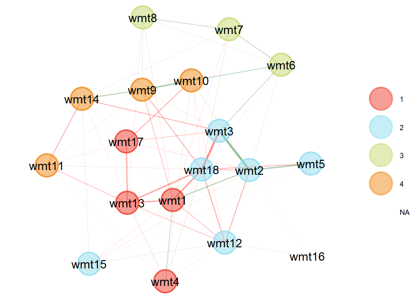
EGAnet also implements random-intercept Exploratory Graph Analysis (riEGA), allowing dimensionality to be explored after separating a general response-style component (Golino & Christensen, 2023).
Warning: Some variables did not belong to a dimension: wmt16

Use caution: These variables have been removed from the TEFI calculation
The random-intercept model converged. Wording effects likely. Results are only valid if data are [4;munrecoded[0m.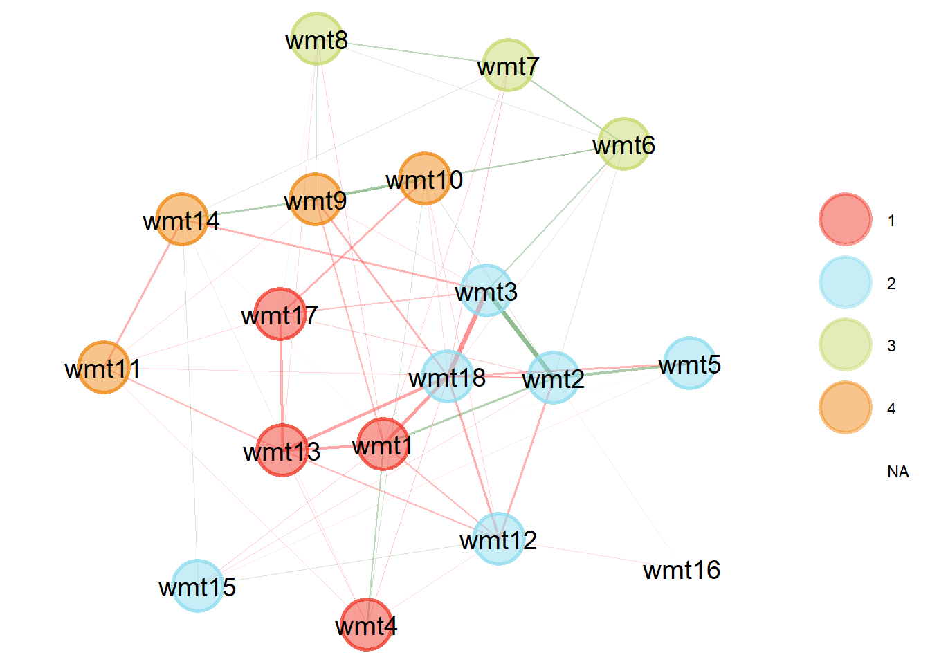
The resulting structure can be bootstrapped:
Show bootstrap riEGA code
Warning: Some variables did not belong to a dimension: wmt16

Use caution: These variables have been removed from the TEFI calculation
The random-intercept model converged. Wording effects likely. Results are only valid if data are [4;munrecoded[0m.Warning in order(as.numeric(names(dimension_stability))): NAs introduzidos por
coerção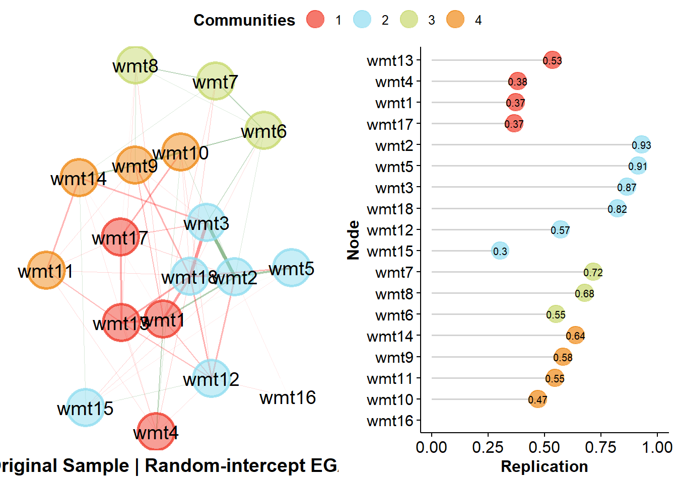
Inspect the distribution of recovered dimensions:
Model: GLASSO (EBIC)
Correlations: auto
Algorithm:  Walktrap
Unidimensional Method:  Louvain

----

EGA Type: riEGA
Bootstrap Samples: 500 (Parametric)

                1     2     3     4     5     6
Frequency:  0.002 0.212 0.358 0.298 0.108 0.022

Median dimensions: 3 [1.02, 4.98] 95% CI
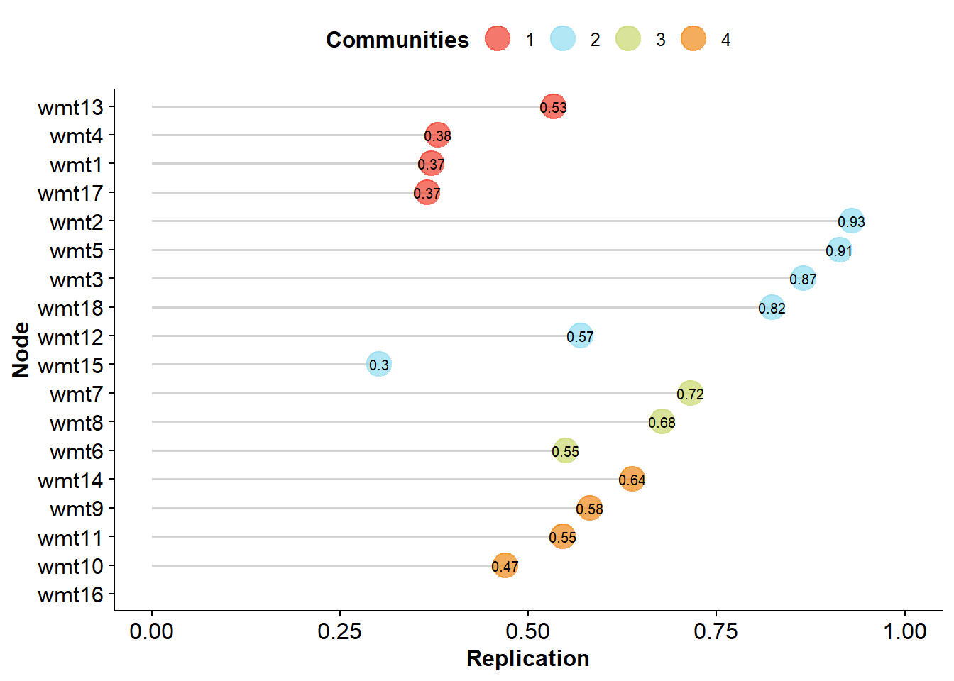
and item stability:
EGA Type: riEGA
Bootstrap Samples: 500 (Parametric)

Proportion Replicated in Dimensions:

 wmt1  wmt2  wmt3  wmt4  wmt5  wmt6  wmt7  wmt8  wmt9 wmt10 wmt11 wmt12 wmt13
0.372 0.930 0.866 0.380 0.914 0.550 0.716 0.678 0.582 0.470 0.546 0.570 0.534
wmt14 wmt15 wmt16 wmt17 wmt18
0.638 0.302    NA 0.366 0.824
Network loadings can also be inspected:
The default 'loading.method' has changed to "revised" in {EGAnet} version >= 2.0.7.

For the previous default (version <= 2.0.6), use `loading.method = "original"` 1 2 3 4 NA
wmt1 0.2444576992 0.247258716 -0.099319925 -0.06883984 NaN
wmt17 0.1370056212 -0.074162443 -0.002957388 -0.07293878 NaN
wmt4 0.1259691396 0.047716919 0.000000000 0.03862790 NaN
wmt13 -0.3415948996 0.135160655 -0.027042546 0.06328015 NaN
wmt2 0.0375993097 0.429380347 0.030746520 0.06192070 -Inf
wmt3 -0.0525405946 0.347886178 0.081803378 -0.09782837 NaN
wmt5 0.0009795657 0.169016832 0.000000000 0.00000000 NaN
wmt12 -0.0199842313 -0.014839834 0.000000000 -0.02866109 -Inf
wmt15 -0.0426694270 -0.052333808 0.000000000 0.02031100 NaN
wmt18 -0.0662899852 -0.222850866 -0.098300041 -0.10194983 NaN
wmt7 -0.0291471025 0.037039191 0.285159251 0.01822694 NaN
wmt6 0.0000000000 0.066980959 0.188532984 0.10200772 NaN
wmt8 -0.0206784252 0.000000000 0.166287494 0.03269760 NaN
wmt9 -0.0626554022 0.049519634 0.102199182 0.29389997 NaN
wmt14 -0.0135862414 -0.072701567 0.026287115 0.22635876 NaN
wmt10 -0.0664420920 0.058653950 0.092074489 0.14410384 NaN
wmt11 0.0162793907 -0.017457853 0.000000000 -0.14361692 NaN
wmt16 0.0000000000 0.007163448 0.000000000 0.00000000 NaNLow item stability or unexpected network loadings should trigger substantive investigation. They should not automatically initiate an iterative delete-and-rerun procedure until every statistic exceeds a fixed cutoff.
An unstable item can represent ambiguous wording, construct overlap, sampling uncertainty, or a genuine boundary between dimensions. Removing it solely to increase stability can narrow the construct and capitalize on the current sample.
12.3.1 Optional CFA follow-up
A factor model based on the EGA structure can be fitted with EGAnet:
[1] "wmt1"  "wmt4"  "wmt13" "wmt17"
[1] "wmt2"  "wmt3"  "wmt5"  "wmt12" "wmt15" "wmt18"
[1] "wmt6" "wmt7" "wmt8"
[1] "wmt9"  "wmt10" "wmt11" "wmt14"
Warning: lavaan->lav_parse_check_relational():
having identifiers with spaces ('Fat 1') is deprecated at line 1, pos 1
Fat 1 =~ wmt1 + wmt4 + wmt13 + wmt17
^
Warning: lavaan->lav_parse_check_relational():
having identifiers with spaces ('Fat 1') is deprecated at line 1, pos 1
Fat 1 =~ wmt1 + wmt4 + wmt13 + wmt17
^
Warning: lavaan->lav_parse_check_relational():
having identifiers with spaces ('Fat 1') is deprecated at line 1, pos 1
Fat 1 =~ wmt1 + wmt4 + wmt13 + wmt17
^
Warning: lavaan->lav_parse_check_relational():
having identifiers with spaces ('Fat 1') is deprecated at line 1, pos 1
Fat 1 =~ wmt1 + wmt4 + wmt13 + wmt17
^Warning: lavaan->lav_parse_check_relational():
having identifiers with spaces ('Fat 2') is deprecated at line 2, pos 2
Fat 2 =~ wmt2 + wmt3 + wmt5 + wmt12 + wmt15 + wmt18
^
Warning: lavaan->lav_parse_check_relational():
having identifiers with spaces ('Fat 2') is deprecated at line 2, pos 2
Fat 2 =~ wmt2 + wmt3 + wmt5 + wmt12 + wmt15 + wmt18
^
Warning: lavaan->lav_parse_check_relational():
having identifiers with spaces ('Fat 2') is deprecated at line 2, pos 2
Fat 2 =~ wmt2 + wmt3 + wmt5 + wmt12 + wmt15 + wmt18
^
Warning: lavaan->lav_parse_check_relational():
having identifiers with spaces ('Fat 2') is deprecated at line 2, pos 2
Fat 2 =~ wmt2 + wmt3 + wmt5 + wmt12 + wmt15 + wmt18
^
Warning: lavaan->lav_parse_check_relational():
having identifiers with spaces ('Fat 2') is deprecated at line 2, pos 2
Fat 2 =~ wmt2 + wmt3 + wmt5 + wmt12 + wmt15 + wmt18
^
Warning: lavaan->lav_parse_check_relational():
having identifiers with spaces ('Fat 2') is deprecated at line 2, pos 2
Fat 2 =~ wmt2 + wmt3 + wmt5 + wmt12 + wmt15 + wmt18
^Warning: lavaan->lav_parse_check_relational():
having identifiers with spaces ('Fat 3') is deprecated at line 3, pos 2
Fat 3 =~ wmt6 + wmt7 + wmt8
^
Warning: lavaan->lav_parse_check_relational():
having identifiers with spaces ('Fat 3') is deprecated at line 3, pos 2
Fat 3 =~ wmt6 + wmt7 + wmt8
^
Warning: lavaan->lav_parse_check_relational():
having identifiers with spaces ('Fat 3') is deprecated at line 3, pos 2
Fat 3 =~ wmt6 + wmt7 + wmt8
^Warning: lavaan->lav_parse_check_relational():
having identifiers with spaces ('Fat 4') is deprecated at line 4, pos 2
Fat 4 =~ wmt9 + wmt10 + wmt11 + wmt14
^
Warning: lavaan->lav_parse_check_relational():
having identifiers with spaces ('Fat 4') is deprecated at line 4, pos 2
Fat 4 =~ wmt9 + wmt10 + wmt11 + wmt14
^
Warning: lavaan->lav_parse_check_relational():
having identifiers with spaces ('Fat 4') is deprecated at line 4, pos 2
Fat 4 =~ wmt9 + wmt10 + wmt11 + wmt14
^
Warning: lavaan->lav_parse_check_relational():
having identifiers with spaces ('Fat 4') is deprecated at line 4, pos 2
Fat 4 =~ wmt9 + wmt10 + wmt11 + wmt14
^Warning: lavaan->lav_object_post_check():
covariance matrix of latent variables is not positive definite ; use
lavInspect(fit, "cov.lv") to investigate.
Warning: lavaan->lav_object_post_check():
covariance matrix of latent variables is not positive definite ; use
lavInspect(fit, "cov.lv") to investigate.
Warning: lavaan->lav_object_post_check():
covariance matrix of latent variables is not positive definite ; use
lavInspect(fit, "cov.lv") to investigate.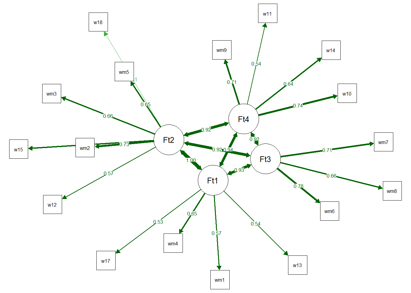
and inspected with lavaan:
Warning: lavaan->lav_object_post_check():
   covariance matrix of latent variables is not positive definite ; use
   lavInspect(fit, "cov.lv") to investigate.
Warning: lavaan->lav_object_post_check():
   covariance matrix of latent variables is not positive definite ; use
   lavInspect(fit, "cov.lv") to investigate.
Warning: lavaan->lav_object_post_check():
   covariance matrix of latent variables is not positive definite ; use
lavInspect(fit, "cov.lv") to investigate. npar fmin
40.000 0.098
chisq df
231.983 113.000
pvalue chisq.scaled
NA 323.795
df.scaled pvalue.scaled
113.000 0.000
chisq.scaling.factor baseline.chisq
0.741 11168.058
baseline.df baseline.pvalue
136.000 NA
baseline.chisq.scaled baseline.df.scaled
7229.787 136.000
baseline.pvalue.scaled baseline.chisq.scaling.factor
0.000 1.555
cfi tli
0.989 0.987
cfi.scaled tli.scaled
0.970 0.964
cfi.robust tli.robust
0.888 0.865
nnfi rfi
0.987 0.975
nfi pnfi
0.979 0.814
ifi rni
0.989 0.989
nnfi.scaled rfi.scaled
0.964 0.946
nfi.scaled pnfi.scaled
0.955 0.794
ifi.scaled rni.scaled
0.970 0.970
nnfi.robust rni.robust
0.865 0.888
rmsea rmsea.ci.lower
0.030 0.024
rmsea.ci.upper rmsea.ci.level
0.035 0.900
rmsea.pvalue rmsea.close.h0
1.000 0.050
rmsea.notclose.pvalue rmsea.notclose.h0
0.000 0.080
rmsea.scaled rmsea.ci.lower.scaled
0.040 0.035
rmsea.ci.upper.scaled rmsea.pvalue.scaled
0.045 1.000
rmsea.notclose.pvalue.scaled rmsea.robust
0.000 0.082
rmsea.ci.lower.robust rmsea.ci.upper.robust
0.072 0.093
rmsea.pvalue.robust rmsea.notclose.pvalue.robust
0.000 0.660
rmr rmr_nomean
0.053 0.056
srmr srmr_bentler
0.056 0.053
srmr_bentler_nomean crmr
0.056 0.056
crmr_nomean srmr_mplus
0.059 NA
srmr_mplus_nomean gfi
NA 0.988
gfi.ci.lower gfi.ci.upper
0.984 0.992
gfi.ci.level gfi.robust
0.900 0.917
gfi.ci.lower.robust gfi.ci.upper.robust
0.897 0.936
cn_05 cn_01
709.467 771.074
gfi_lisrel agfi_lisrel
0.983 0.977
pgfi mfi
0.726 0.951
wrmr
1.231
attr(,"scaled.test")
[1] "scaled.shifted"If the structure was discovered and evaluated in the same sample, the CFA is a follow-up description rather than independent confirmation. Cross-validation in a separate sample provides stronger evidence.
Latent scores from the fitted CFA can be estimated as follows:
13 A Practical Acquiescence Checklist
| Stage | Question |
|---|---|
| Item design | Do the positive and opposite-key items represent genuinely opposite content? |
| Response format | Could the category labels themselves encourage agreement? |
| Data structure | Do positive and reverse-keyed items form separate method clusters? |
| Model | Is acquiescence represented independently from substantive factors? |
| Magnitude | Does the response-style component explain nontrivial variance? |
| Stability | Are item assignments stable when acquiescence is controlled? |
| Interpretation | Does control improve substantive interpretability rather than only numerical fit? |
14 Concluding Remarks
Acquiescence is deceptively simple to define but difficult to control. The basic tendency—agreement regardless of content—can create systematic covariance across questionnaire items. Oppositely keyed items make this tendency observable, but they can also introduce their own wording and comprehension effects.
The strongest approach is therefore not to treat reverse wording as a universal remedy. Item design, response format, and statistical modeling should work together. Random-intercept models and related response-bias methods can separate a general endorsement tendency from substantive traits, but the separation is only as defensible as the assumptions that identify the response-style component.
In practical work, the objective is not to obtain a questionnaire that is statistically free of every response tendency. It is to understand which parts of the observed covariance can plausibly be attributed to the target construct and which may arise from the way respondents use the response scale.