2 Classical Test Theory
Psychological and educational assessment depends heavily on scores. A student receives a score on an examination, a patient receives a score on a symptom scale, and a research participant receives a score on a questionnaire. We often interpret these numbers as indicators of an underlying attribute, such as knowledge, anxiety, self-esteem, or well-being. Yet the same person would rarely obtain exactly the same score if the assessment were repeated.
Suppose a student takes equivalent versions of the same examination on many occasions and obtains scores such as 74, 78, 75, 81, 76, and 73. Which of these is the student’s “true” score? Classical test theory (CTT) provides one influential way to formalize this problem. Its central idea is simple: an observed score reflects both a stable component and measurement error (Brennan, 2011; Lord & Novick, 1968).
NoteChapter roadmap
In this chapter, we move from the basic CTT decomposition to reliability, the standard error of measurement, confidence intervals, test length, classical item analysis, and a worked example in R. The final section also makes explicit what CTT can—and cannot—tell us about psychological measurement.
2.1 Why Do Scores Vary?
Variation in observed scores does not necessarily imply that the attribute itself has changed. A person’s performance can be influenced by temporary factors such as fatigue, attention, guessing, the particular items sampled, environmental distractions, or other sources of random variation. CTT provides a framework for describing how this uncertainty affects observed scores (Lord & Novick, 1968; Pasquali, 2017).
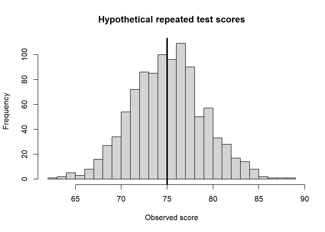
A useful way to develop intuition is to imagine an indefinitely large number of hypothetical replications of the same measurement procedure under the conditions that define the test. The observed score can vary from one replication to another, but the center of this hypothetical distribution is treated as the person’s true score.
The vertical line represents the expected score across hypothetical replications. Individual observed scores fluctuate around that value.
2.2 The Classical Test Theory Model
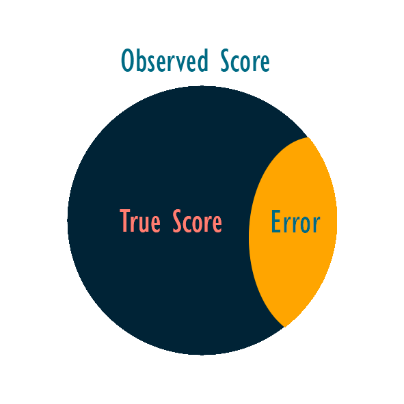
The basic CTT decomposition is
\[ X = T + E, \]
where
- \(X\) is the observed score,
- \(T\) is the true score, and
- \(E\) is the error score.
The relationship is illustrated in Figure 2.2.
2.2.1 Observed score
The observed score, \(X\), is the score actually produced by the measurement procedure. Depending on the assessment, it might be a sum, mean, weighted composite, or another scoring function.
2.2.2 True score
In CTT, the true score is formally defined as the expected observed score across hypothetical replications of the measurement procedure (Brennan, 2011; Lord & Novick, 1968):
\[ T = \mathbb{E}(X). \]
This definition is important because the CTT true score should not be equated automatically with a person’s “real ability,” “real anxiety,” or the construct itself. It is a property of the measurement procedure. A test can produce highly consistent true scores while still measuring the wrong attribute or supporting an invalid interpretation.
This distinction connects directly to the discussion of validity in Chapter 1: reliability concerns the consistency or precision of scores, whereas validity concerns the interpretation and use of those scores.
2.2.3 Error score
For a particular administration,
\[ E = X - T. \]
The error score represents the deviation of the observed score from the person’s expected score under the CTT replication framework. It is not directly observed because \(T\) is itself unobserved.
WarningRandom error is not the same as systematic bias
A systematic influence that persists across hypothetical replications can become part of the expected score \(T\) rather than appearing as random error \(E\). For example, if an item systematically disadvantages a group in the same way each time it is administered, high reliability does not make that bias disappear. A measure can therefore be highly reliable and still support an invalid interpretation (Brennan, 2011; Lord & Novick, 1968).
2.3 Assumptions of the CTT Decomposition
The equation \(X=T+E\) becomes useful through the definitions and assumptions attached to it. The fundamental expectation is
\[ \mathbb{E}(E)=0. \]
Because \(T=\mathbb{E}(X)\), errors average to zero over the hypothetical replications that define the measurement procedure. A positive error on one occasion is, in expectation, balanced by negative errors on other occasions.
A second important result is that true scores and errors are uncorrelated in the classical model:
\[ \operatorname{Cov}(T,E)=0. \]
When parallel measurements are considered, CTT additionally assumes that their error scores are uncorrelated:
\[ \operatorname{Cov}(E,E')=0. \]
These assumptions allow the variance of observed scores to be decomposed:
\[ \sigma_X^2 = \sigma_T^2 + \sigma_E^2. \]
Thus, observed-score variance contains both systematic between-person variation represented by true scores and variation attributable to measurement error (Brennan, 2011; Lord & Novick, 1968).
ImportantCTT is not an ordinary regression model
The expression \(X=T+E\) resembles a regression decomposition, but the analogy is limited. Neither \(T\) nor \(E\) is directly observed, and \(E\) should not simply be interpreted as an ordinary fitted-model residual. The CTT components receive their meaning from the definitions and replication assumptions imposed on the measurement procedure (Brennan, 2011).
2.4 From Measurement Error to Reliability
Reliability describes how much of the observed-score variance is attributable to true-score variance rather than error variance. In CTT,
\[ \rho_{XX'} = \frac{\sigma_T^2}{\sigma_X^2} = \frac{\sigma_T^2} {\sigma_T^2+\sigma_E^2}. \]
Under the assumptions of parallel forms, reliability can also be expressed as the correlation between two parallel measurements:
\[ \rho_{XX'}=\operatorname{Cor}(X,X'). \]
Reliability approaches 1 as error variance becomes small relative to true score variance. Conversely, reliability decreases as error variance becomes large relative to true-score variance (Brennan, 2011; Lord & Novick, 1968).
2.4.1 Reliability is a property of scores in a population
Reliability is sometimes discussed as if it were a permanent characteristic of an instrument—for example, “this scale has a reliability of .85.” This shorthand can be misleading.
Because reliability is a variance ratio,
\[ \rho_{XX'} = \frac{\sigma_T^2} {\sigma_T^2+\sigma_E^2}, \]
its magnitude depends partly on the amount of true-score variability in the population being studied. If a sample is highly homogeneous, \(\sigma_T^2\) may be small and reliability can decrease even when the measurement procedure itself has not changed. A more heterogeneous sample can produce a larger reliability coefficient because there is more between-person variance to distinguish (Brennan, 2011; Lord & Novick, 1968).
For this reason, reliability should normally be estimated and reported for the sample and score use under investigation rather than treated as a fixed property inherited from a previous validation study.
2.5 Parallel, Tau-Equivalent, and Congeneric Measures
Different reliability coefficients rely on different measurement assumptions. It is useful to distinguish three common models (Graham, 2006; McDonald, 1999).
2.5.1 Parallel measures
Parallel measures are the most restrictive. They have the same true scores and equal error variances. In simplified notation,
\[ X_1=T+E_1, \qquad X_2=T+E_2, \]
with
\[ \sigma_{E_1}^2=\sigma_{E_2}^2. \]
2.5.2 Tau-equivalent measures
Tau-equivalent measures relax some of the parallel-form restrictions. Their expected scores may differ by additive constants while reflecting the same underlying true-score variation. In a factor-model interpretation, tau-equivalence corresponds approximately to items having equal loadings on the common factor while allowing their intercepts and error variances to differ.
2.5.3 Congeneric measures
Congeneric measurement is more flexible:
\[ X_j=\alpha_j+\lambda_jT+E_j. \]
Different items can have different intercepts, different relationships with the common attribute, and different error variances. This is often a more realistic representation of psychological scales, where some items are stronger indicators than others (Graham, 2006; McDonald, 1999).
These distinctions matter because a reliability coefficient can perform well under one model and poorly under another.
2.6 Ways of Estimating Reliability
The appropriate reliability estimate depends on the source of measurement error that the researcher wants to evaluate.
2.6.1 Test–retest reliability
Test–retest reliability examines score stability across occasions. The same assessment is administered to the same people at different times, and the association between scores is evaluated.
This design is useful when temporal instability is a relevant source of measurement error. However, low test–retest correlations can reflect actual change in the attribute, measurement error, or both. The time interval and the substantive stability of the construct therefore matter.
2.6.2 Alternate-forms reliability
Alternate-form reliability compares scores from different versions of the same assessment. If the forms are genuinely parallel, their correlation estimates CTT reliability. In practice, constructing truly parallel forms is difficult because forms can differ in difficulty, content sampling, or error variance (Brennan, 2011).
2.6.3 Split-half reliability
A test can also be divided into two parts and the association between the half-test scores examined. Because each half is shorter than the complete test, the raw correlation between halves underestimates the reliability of the full-length test. The Spearman–Brown formula corrects for this difference (Brown, 1910; Spearman, 1910).
2.6.4 Internal-consistency coefficients
Internal-consistency coefficients estimate reliability using information from the items obtained in a single administration. The best-known example is coefficient alpha.
2.7 Coefficient Alpha
For a test with \(k\) items, coefficient alpha can be written as
\[ \alpha = \frac{k}{k-1} \left( 1- \frac{\sum_{j=1}^{k}\sigma_j^2} {\sigma_X^2} \right), \]
where \(\sigma_j^2\) is the variance of item \(j\) and \(\sigma_X^2\) is the variance of the total score (Cronbach, 1951).
Alpha became the most frequently reported internal-consistency coefficient in psychology, but several common interpretations are incorrect (Cortina, 1993; Sijtsma, 2009).
WarningWhat alpha does not tell you
A large alpha does not demonstrate that a scale is unidimensional, does not establish construct validity, and does not mean that a score is “90% accurate” when \(\alpha=.90\). Alpha is influenced by the number of items, item covariances, and the assumptions of the score model. Under essential tau-equivalence and uncorrelated errors, alpha can represent score reliability; when these assumptions are violated, its relationship with reliability becomes less straightforward (Graham, 2006; Sijtsma, 2009).
A particularly important consequence is that adding highly redundant items can increase alpha without improving the conceptual breadth or validity of the instrument. The goal of scale development should therefore not be to maximize alpha mechanically.
2.8 From Alpha to Omega
When items are congeneric and have different factor loadings, a factor-model-based reliability coefficient such as McDonald’s omega can often provide a more appropriate estimate of composite-score reliability (Dunn et al., 2014; McDonald, 1999).
A simplified expression for omega for a unidimensional factor model is
\[ \omega = \frac{\left(\sum_{j=1}^{k}\lambda_j\right)^2 \sigma_F^2} { \left(\sum_{j=1}^{k}\lambda_j\right)^2\sigma_F^2 + \sum_{j=1}^{k}\theta_j }, \]
where \(\lambda_j\) are factor loadings, \(\sigma_F^2\) is factor variance, and \(\theta_j\) are error variances.
Omega is not simply “a better alpha” in every circumstance. It relies on a measurement model, and its interpretation depends on the adequacy of that model. Conceptually, this also means that omega begins to move beyond the simplest CTT framework and toward the latent-variable models discussed later in this book (Dunn et al., 2014; McDonald, 1999).
2.9 Standard Error of Measurement
Reliability is a population-level variance ratio. For psychological assessment, however, we often want to know how much uncertainty surrounds an individual observed score.
The standard error of measurement (SEM) expresses measurement error in the metric of the test (Harvill, 1991):
\[ SEM = SD_X\sqrt{1-\rho_{XX'}}. \]
Suppose a scale has
\[ SD_X=10 \]
and
\[ \rho_{XX'}=.84. \]
Then
\[ SEM = 10\sqrt{1-.84} = 4. \]
An SEM of 4 means that the standard deviation of measurement errors is approximately four score points under the assumptions of the model.
2.9.1 Confidence intervals around scores
A common approximate interval is
\[ X \pm z(SEM). \]
For a 95% normal-theory interval,
\[ X \pm 1.96(SEM). \]
If a participant obtains \(X=70\) and \(SEM=4\), the approximate interval is
\[ 70 \pm 1.96(4) = [62.16,\;77.84]. \]
The interval communicates an important fact that is often hidden when a single score is reported: observed scores are estimates with uncertainty, not perfectly precise measurements.
Harvill (1991) also emphasizes that a single SEM assumes approximately constant measurement precision across score levels. In practice, conditional standard errors may differ across the score distribution, an issue that becomes especially important in item response theory.
TipReliability and SEM answer different questions
Reliability: How well can the test distinguish people in a population?
SEM: How much measurement uncertainty is expressed in the units of the observed score?
A reliability coefficient can therefore look impressive while the SEM remains too large for a particular individual-level decision.
2.10 Test Length and the Spearman–Brown Formula
Longer tests often have higher reliability because additional items can increase systematic score variance relative to random item-sampling error. The Spearman–Brown prophecy formula describes the expected reliability after multiplying test length by a factor \(k\) (Brown, 1910; Spearman, 1910):
\[ \rho_{\text{new}} = \frac{k\rho_{\text{old}}} {1+(k-1)\rho_{\text{old}}}. \]
Suppose a test has reliability .70 and its length is doubled (\(k=2\)):
\[ \rho_{\text{new}} = \frac{2(.70)} {1+(2-1)(.70)} = .824. \]
The formula is useful for planning, but it assumes that the added items behave like the existing items. Adding poor, redundant, or construct-irrelevant items merely to increase reliability is not a sound validation strategy.
2.11 Classical Item Analysis
CTT can also be used to inspect how individual items contribute to a score (Crocker & Algina, 1986; Pasquali, 2017).
For each item, researchers commonly examine:
- Item mean or endorsement rate. For dichotomous achievement items, this is often interpreted as item difficulty. For rating scales, the mean indicates where responses tend to fall on the response scale.
- Item variance. Items with almost no response variability contribute little to differentiating respondents in that sample.
- Corrected item–total correlation. This correlates an item with the total score computed without that item. It provides information about whether the item behaves consistently with the rest of the composite.
- Reliability after item deletion. This can identify items that behave differently from the remainder of the scale, but it should not be used as an automatic item-deletion algorithm.
WarningDo not let reliability choose the construct
Deleting items simply because alpha increases can narrow the content domain and damage validity. Item statistics must be interpreted together with construct definitions, response-process evidence, and the intended use of scores. A psychometrically homogeneous test is not necessarily a valid test.
2.12 A Worked Example in R
The following example simulates ten continuous items that share a common person component plus item-specific error. The code calculates coefficient alpha directly from its CTT formula and then computes the SEM for the total score.
set.seed(2026)

n_people <- 500
n_items <- 10

# Common person component
person_component <- rnorm(n_people, mean = 0, sd = 1)

# Each item contains the common component plus item-specific error
items <- replicate(
  n_items,
  person_component + rnorm(n_people, mean = 0, sd = 0.80)
)

colnames(items) <- paste0("item_", seq_len(n_items))

# Total score
total_score <- rowSums(items)

# Coefficient alpha from the variance formula
alpha_ctt <- function(data) {
  k <- ncol(data)
  item_variances <- apply(data, 2, var)
  total_variance <- var(rowSums(data))

  (k / (k - 1)) *
    (1 - sum(item_variances) / total_variance)
}

alpha_estimate <- alpha_ctt(items)

# Standard error of measurement
score_sd <- sd(total_score)

sem_estimate <- score_sd * sqrt(1 - alpha_estimate)

alpha_estimate
[1] 0.9397648[1] 2.527688The example is deliberately simple: the data are continuous, complete, and generated from a common-component model. Real psychological data may be ordinal, multidimensional, locally dependent, or incomplete. In those situations, reliability estimation should be chosen to match the measurement model rather than applied mechanically.
2.12.1 Seeing reliability as a variance ratio
We can also simulate two genuinely parallel measurements:
set.seed(2026)

n <- 2000

T <- rnorm(n, mean = 50, sd = 10)
E1 <- rnorm(n, mean = 0, sd = 5)
E2 <- rnorm(n, mean = 0, sd = 5)

X1 <- T + E1
X2 <- T + E2

# Reliability from the CTT variance decomposition
reliability_variance <- var(T) / var(X1)

# Reliability estimated as the correlation of parallel forms
reliability_parallel <- cor(X1, X2)

reliability_variance
[1] 0.8171529[1] 0.7745723With a sufficiently large sample, the two quantities should be similar. The simulation makes explicit why the correlation of parallel forms can estimate reliability: both forms share the same true-score component while their errors are independent.
2.13 What CTT Can—and Cannot—Tell Us
CTT remains useful because it provides a compact language for reasoning about score precision. Its simplicity is also the source of several limitations.
| CTT can help us ask… | CTT alone cannot establish… |
|---|---|
| How much observed-score variance is associated with measurement error? | What psychological construct the score actually represents |
| How consistently does a score distinguish people in this population? | That the interpretation of the score is valid |
| How much uncertainty surrounds an observed score? | That measurement precision is equal at every trait level |
| How might test length affect reliability? | That additional items improve construct representation |
| Which items behave consistently with a composite? | That the items are unidimensional or causally produced by one latent variable |
A particularly important limitation is that CTT is primarily test-score centered. Item and person characteristics are not separated in the same way they are in item response theory. Reliability and item statistics can therefore change across populations, and the model does not directly describe how measurement precision varies along a latent trait continuum.
At the same time, more complicated models do not eliminate the fundamental problems discussed in Chapter 1. A factor model or IRT model can provide a richer representation of measurement, but statistical fit alone still cannot establish what respondents understood, whether test content adequately represents the construct, or whether the resulting score interpretation is defensible.
2.14 Concluding Remarks
The most important insight of CTT is not the equation \(X=T+E\) itself, but the recognition that an observed score is an imperfect measurement. Reliability formalizes the relative contribution of measurement error to score variability, while the SEM translates that uncertainty back into the metric used to interpret individual scores.
The framework also imposes useful discipline on score interpretation. The CTT true score is an expected score under a specified replication framework—not the psychological construct itself. Reliability therefore cannot substitute for validity, and a highly reliable score can still be systematically biased or substantively meaningless.
This distinction will become increasingly important as we move from CTT to latent-variable and item-level measurement models. Those approaches relax some of CTT’s restrictions and allow more detailed questions about items, persons, and measurement precision. They do not, however, remove the need to ask the central question introduced in the previous chapter: What does this score mean, and what evidence justifies that interpretation?