4 Measurement Theory: Why it is Possible to Measure Psychological Phenomena
Sometimes, on days of perfect and exact light,
When things are as real as they can possibly be,
I slowly ask myself
Why I even bother to attribute Beauty to things.
Does a flower really have beauty?
Does a fruit really have beauty?
No: they have only color and form
And existence.
Beauty is the name of something that doesn’t exist
But that I give to things in exchange for the pleasure they give me.
It means nothing.
So why do I say about things: they’re beautiful?
Yes, even I, who live only off living,
Am unwittingly visited by the lies of men
Concerning things that simply exist.
Concerning things,
How hard to be just what we are and see nothing but the visible!
— Fernando Pessoa
The numerical representation of psychological constructs is central to psychometrics, but assigning numbers is not automatically the same as measurement. Measurement theory asks a deeper question: what must be true about an attribute before numerical operations on its scores are scientifically meaningful?
This chapter introduces that question historically and conceptually. The goal is not to replace psychometric modeling, but to clarify the assumptions that make quantitative interpretations possible.
We will move through six connected ideas:
- the objective of psychometrics;
- the historical debate about quantity and measurement;
- what it means for a variable to be ordered and additive;
- additive conjoint measurement (ACM);
- the debate about whether Rasch modeling entails measurement; and
- approaches for testing measurement axioms empirically.
4.1 The Objective of Psychometrics
Psychometrics is the branch of psychology concerned with quantifying and measuring mental attributes, behavior, performance, feelings, and related phenomena. Yet there is an important disagreement about whether common psychometric procedures truly establish measurement.
As explained by Sijtsma (2012), Michell (2000, 2004, 2008), and Kyngdon (2008b, 2008a), standard psychometric practice may be inadequate for demonstrating that psychological attributes are quantitative. From this perspective, additive conjoint measurement provides a stronger foundation (Luce & Tukey, 1964). Sijtsma (2012) notes that taking this position seriously would demand major changes in contemporary psychology and could substantially slow current research. A reasonable response is to ask whether slowing down is necessarily undesirable if doing so improves the foundations of future measurement.
On the other hand, Borsboom & Mellenbergh (2004) and Borsboom & Zand Scholten (2008) argue that modern psychometrics—particularly item response theory (IRT) (Linden & Hambleton, 1997)—already provides useful tools for psychological measurement. The central tension is therefore between fitting a statistical measurement model and demonstrating that the attribute itself has the quantitative structure assumed by that model.
A statistical model can prescribe numerical relationships among scores. Measurement theory asks whether the empirical attribute being represented actually supports those numerical relationships. These are related, but not identical, questions.
4.2 Dr. Jekyll and Mr. Hyde: Measurement and Validity
When we measure an attribute, we associate empirical properties with numbers or other mathematical entities in such a way that relevant relationships among the objects are faithfully represented numerically (Krantz et al., 1971). In psychological assessment, this problem is closely connected to validity because the interpretation of test scores depends on what those numerical representations are taken to mean (American Educational Research Association et al., 2014; Borsboom, 2005).
As Bringmann & Eronen (2016) note, physical measurement rarely appears in books, manuals, or monographs on measurement and measurement theory in psychology (for example, American Educational Research Association et al., 2014; Borsboom, 2005; Kline, 2000; McDonald, 1999). In the 2014 edition of Standards for Educational and Psychological Testing, validity is the first topic discussed and is characterized as “the most fundamental consideration in test development and test evaluation” (American Educational Research Association et al., 2014, p. 11). According to a classical definition, validity refers to the extent to which a test or instrument measures what it is intended to measure (Kline, 2000, p. 17; McDonald, 1999, p. 197), although contemporary validity theory contains several competing formulations (see Newton & Shaw, 2013). One prominent approach is Messick’s unified treatment of validity (Messick, 1989), which focuses on the appropriateness of the inferences psychologists make from test results. Argument-based approaches developed by Kane likewise frame validation as the process of building and evaluating evidence-based arguments for score interpretations and uses (Kane, 2001, 2006, 2013).
However, approaches to validity ultimately depend on some relationship between a construct and the scores used to represent it. This makes the quantification of psychological phenomena a central issue for psychometric research. I argue that the lack of empirical foundations for psychological measurement is “Mr. Hyde” of psychometrics, a monster for some researchers who, at the same time, is “Dr. Jekyll”, one of the many sources of validity of psychological instruments. This view aligns with Michell (2000), who describes this way of doing psychometrics as “pathological.”
Validity asks whether interpretations and uses of scores are justified. Measurement theory adds a more basic question: do the empirical relationships represented by those scores justify the numerical structure we use?
4.3 History of Psychological Measurement
Before following the historical discussion in detail, the main shift can be summarized as follows.
| Period / thinker | Central idea | Relevance to measurement |
|---|---|---|
| Pythagoras and Plato | Nature is fundamentally mathematical | Encouraged the idea that reality can be represented quantitatively |
| Aristotle | Quantities and qualities are different kinds of attributes | Additive structure distinguishes quantities from qualities |
| Galileo, Newton, Kant, Kelvin | Mathematics became increasingly tied to scientific explanation | Strengthened the quantitative imperative in science |
| Early psychologists | Scientific status became associated with experiment and measurement | Psychology increasingly adopted quantitative methods |
| S. S. Stevens | Measurement is the assignment of numbers according to rules | Broadened the meaning of measurement beyond classical quantity |
| Representational measurement theory | Numerical representation must preserve empirical structure | Reintroduced the question of what makes numerical representation meaningful |
The debate behind what Michell later called the pathology of psychometrics began long before psychometrics existed. Pythagoras is commonly associated with the claim that “All things are made of numbers.” This is a strong assumption: it suggests that the fundamental structure of processes in nature is quantitative. In Timaeus, Plato continues saying the same thing, saying that all things are composed of the four basic elements (earth, fire, air, and water), which, in turn, are formed by polyhedra. He continues this logic, stating that polyhedra are made of triangles, which are reducible to lines and angles, and numbers.
Aristotle offered an important counterpoint to this reduction of everything to quantity. Aristotle recognized that there are quantities (numbers, sizes, areas, etc.), but there are also qualities. These qualities are not quantitative, and concern things like colors and aromas. This distinction he said was something observable, where quantitative properties had an additive structure. Qualities did not have such a structure. Thus, he developed qualitative physics.
This disagreement continued between those who treated nature as fundamentally quantitative and those who argued that not every property has quantitative structure. Sometime later, Galileo himself joined the team of Pythagoras and Plato:
[The universe] cannot be read until we have learnt the language and become familiar with the characters in which it is written. It is written in mathematical language, and the letters are triangles, circles, and other geometrical figures, without which means it is humanly impossible to comprehend a single word. (Galilei, 1864)
You can see the imprint of this speech to this day. People keep claiming that everything can be expressed in mathematical terms. Of course, if you number everything you associate it with mathematics. But what lies behind this thought is saying that everything in life is quantitatively measurable.
Great contemporaries from the same area as Galileo shared his views, such as Kepler and Descartes. However, this was not what made the quantitative area “win”, and rather the fact that Galileo’s physics dominated European science, taking the focus away from its rival, Aristotle’s physics.
With all this success, Galileo gave birth to the quantitative imperative. With the advent of Newton’s works, which strengthened Galileo’s quantitative views, we increasingly have more philosophers who defend this way of thinking. Kant wrote that
… In any special doctrine of nature there can be only as much proper science as there is mathematics therein. (Kant, 1786, p. 7)
You can see here the birthplace of the thought that all science must be quantitative. It was just in the 19th century that Lord Kelvin (an important physicist), expressed these thoughts more concretely
When you can measure what you are speaking about, and express it in numbers, you know something about it; but when you cannot measure it, when you cannot express it in numbers, your knowledge is of a meagre and unsatisfactory kind: it may be the beginning of knowledge, but you have scarcely, in your thoughts, advanced to the stage of science, whatever the matter may be. (Thomson, 1891, p. 81)
Thus, this speech became the new favorite of the quantitative movement. Pearson, for example, later repeated this quantitative ideal (Pearson, 1978). And like many other areas that wanted to claim to be scientific because of quantitative thinking, psychology was no different. Back when psychology emerged in the nineteenth century, G. Fechner was also influenced by the thinking of the time about the nature of science (Fechner, 1860). Fechner was a physicist who later became interested in psychological issues, such as the intensity of sensations. Although he was not the first person to attempt to measure psychological variables (perhaps it was Nicole Oresme in the 14th century), he proposed measurement methods.
Well, quantitative thinking continued in the progenitors of psychology (in this branch of psychology, in this case). Eugenicist Francis Galton, who influenced and did many studies on psychology, wrote that
…until the phenomena of any branch of knowledge have been subjected to measurement and number, it cannot assume the status and dignity of a science. (Galton, 1879, p. 147)
His assistant and one of the first psychology professors, James McKeen Cattell, followed this line of thought:
Psychology cannot attain the certainty and exactness of the physical sciences, unless it rests on a foundation of experiment and measurement. (Cattell, 1890, p. 373)
Even the creator of Factor Analysis, Charles Spearman, wrote that:
… great as may be the potency of this [the experimental method], or of the preceding methods, there is yet another one so vital that, if lacking it, any study is thought by many authorities not to be scientific in the full sense of the word. This further and crucial method is that of measurement. (Spearman, 1937, p. 89)
E. B. Titchener (1905, pp. xxi–xxii) and Külpe (1895, p. 11) expressed similar views, arguing that mental processes were measurable. Few who claimed that psychology was a science actually questioned the idea that it could be quantitative. This was probably because the status of science could be lost. A psychologist dared to do this: Franz Brentano. He adhered a little to the Aristotelian thoughts.
Mathematics appears to me necessary for the exact treatment of all sciences only because we now in fact find magnitudes in every scientific field. If there were a field in which we encountered nothing of the sort, exact description would be possible even without mathematics. (Brentano, 1874, p. 65)
S. S. Stevens attempted to resolve the tension between those who did and did not consider psychological attributes measurable. Stevens argued that numerical representation need not be restricted to additive quantities and popularized the nominal, ordinal, interval, and ratio scale typology. Across several publications, he defined measurement as the assignment of numbers to objects or events according to rules (Stevens, 1946, 1951, 1959). This is one of the most famous measurement definitions in psychology today. You can find it as the main definition in thousands of psychology and psychometrics books.
However, his definition is empty of meaning. Not only are all things measurable, but also all things that can be numbered are forms of measurement. Furthermore, the distinction between quantitative and qualitative variables vanished. In other words, the variable being quantitative is no longer a characteristic of the variable itself, rather it is a pragmatic issue, decided by the researcher. Steven’s definition confuses two distinct practices: a) measurement (in the classical sense); and b) numerical coding. Measurement involves the discovery of empirical facts of an intrinsic numeric type. b) Numerical coding is simply a cosmetic use in analysis and presentation of something that is not numeric. It is just a symbolic representation of facts.
4.4 How to Move Forward: Defining Quantity
After this historical debate, the key question remains: what is a quantity? What distinguishes a quantitative variable from a non-quantitative one? In the classical framework used here, a quantity must have both an order structure and an additive structure. We can build this idea step by step.
| Concept | Simple question | Example |
|---|---|---|
| Variable | In what respect can objects differ? | height, color, speed |
| Value | Which particular property or relation is present? | 1.80 m, red, 60 km/h |
| Order | Can values be meaningfully ranked? | 6 m > 2 m |
| Additivity | Can differences be combined according to consistent rules? | 2 m + 4 m = 6 m |
All quantitative variables are ordered, but not every ordered variable is quantitative. The additional requirement is an additive structure.
What would be a variable? In general, it is anything relative to which objects can vary. Size is a variable, as different objects have different sizes. Color is a variable, given that we have several colors. Being more detailed about this, the class of variables (size, color, etc.) can only be presented once for each object. Therefore, I do not have two heights at the same time. This is a condition crucial for a variable: not owning the same property more than once. Of course, we can have different properties on the same object, such as being a tall, white, brown-haired person. We have 3 variables (height, race/ethnicity, and hair color). But that’s not all that characterizes a variable.
Relationships also form variables. The difference between properties and relationships is important. Things have uniquely shaped properties, like the size of my pen is one. Relationships involve a plurality of things. If the pen is on a table, then the situation involves both the pen and the table. Another example is speed. The speed of \(X\) relative to \(Y\) is something that involves \(X\) and \(Y\). Of course, the speed of \(X\) relative to \(Y\) is just one. But we can also have another speed, that of \(X\) in relation to \(Z\). This does not mean that \(X\) has more than one speed at the same time, it only has one, but there is also a relationship between the objects \(X\), \(Y\), and \(Z\).
Another important concept is that of value: the properties and relationships that constitute a variable can be called values of that variable. For example, being 6 meters in size is the value of the size variable. Being a woman is the value of the gender variable, and so on. When we say that a quantitative variable is ordered and additive, we are saying that there are ordinal and additive relationships between the values of that variable.
What constitutes an ordered variable? Well, a simple way is to think that 6 meters is greater than 2 meters. We can also think about education, where higher education is more education than secondary education, which in turn is more than elementary education. More concretely, the values of the variables are ordered according to their magnitudes. We use the symbol \(≥\), which means “greater than or at least equal to”, and \(>\) meaning “greater than”. The symbol \(=\) means “equal to” or “identity of the value”. Now let’s go to the mathematics of the thing.
Consider \(X\), \(Y\), and \(Z\) as three values of a variable \(Q\). The order relation must satisfy three properties:
if \(𝑋 ≥ 𝑌\) and \(𝑌 ≥ 𝑍\), then \(𝑋 ≥ 𝑍\) (this property is called transitivity. It means that if \(𝑋\) is greater than or equal to \(Y\), and \(𝑌\) is greater than or equal to \(𝑍\), then \(𝑋\) must be greater than or equal to \(Z\), given the first relations mentioned).
if \(𝑋 ≥ 𝑌\) and \(𝑌 ≥ 𝑋\), then \(𝑋 = 𝑌\) (also called antisymmetry. It means that If \(𝑋\) is greater than \(𝑌\), and \(𝑌\) is greater than \(𝑋\), how can they not be greater than the other at the same time, so they have to be the same).
either \(𝑋 ≥ 𝑌\) or \(𝑌 ≥ 𝑋\) (called strong connectedness; only one variable can be larger, or both are the same).
A relation satisfying these three properties is called a simple order. Thus, \(Q\) is ordinal when \(≥\) forms a simple order over its values. Again, order is necessary for quantity, but it is not sufficient; we also need additivity.
Additivity is represented by a ternary relation such as \(X + Y = Z\). For an ordered variable \(Q\), the additive structure used here requires the following properties:
\(X + (𝑌 + 𝑍) = (𝑋 + 𝑌 ) + 𝑍\) (associativity; i.e., the order of the sum does not affect the value resulting from the sum)
\(𝑋 +𝑌 = 𝑌 +𝑋\) (commutativity; i.e., the order of the operands does not affect the final result).
\(𝑋 ≥ 𝑌\) if and only if \(𝑋 + 𝑍 ≥ 𝑌 + 𝑍\) (monotonicity; that is, if we add the same value on both sides, in \(𝑋\) and \(𝑌\), their order continues in the same direction, where \(𝑋\) is greater than or equal to \(𝑌\)).
If \(𝑋 ≥ 𝑌\) then there is a value \(𝑍\) that makes \(𝑋 = 𝑌 + 𝑍\) (solvability; means that if a value \(𝑋\) is greater than the value \(𝑌\), there is a third value \(𝑍\) which added to \(𝑌\) makes it a value equal to \(𝑋\)).
\(𝑋 + 𝑌 ≥ 𝑋\) (positivity; if \(X\) is increased by a value \(𝑌\), then this result has be greater than the original value of \(𝑋\), given that they are ordinal variables).
there is a natural number \(n\) such as \(n𝑋 ≥ 𝑌\) (where \(1𝑋 = 𝑋\) and \((𝑛+1)𝑋 = 𝑛𝑋+𝑋\) (Archimedean Condition; means that no value \(𝑌\) of the variable is infinitely greater than any other variable \(𝑋\)).
Together, the three ordering conditions and six additive conditions describe the structure of the variable. They do not, by themselves, describe the behavior of the objects that possess values on that variable.
A score can be coded numerically without establishing that the attribute represented by the score satisfies these structural conditions. The measurement-theory question comes before asking whether a statistical model fits the observed data.
Thus, it is not just additivity that a measure lives on. But an important criticism of Michell is how psychometricians do not evaluate their models correctly, at the level of measurement theory. As a result, they assume many things that may or may not be true, requiring testing or theorizing about these created measures. If psychometricians really evaluated the level of measurement of their variables, this would already solve the problem of psychometrics being pathological. We cannot keep assuming things that can be testable, or at least theorized in a more concrete way.
4.5 Additive Conjoint Measurement
The presentation of additive conjoint measurement (ACM) below follows Michell (2014). Luce & Tukey (1964) proposed ACM as a way to establish quantitative structure without requiring physical concatenation. Instead of literally joining objects, ACM evaluates whether ordinal relationships among combinations of variables behave as they should if an underlying quantitative structure exists. This is especially relevant to psychology, where concatenation operations are often unavailable but ordinal comparisons are common.
If the observed ordering of outcomes satisfies specific axioms, then it may be possible to represent the underlying variables numerically in an additive way.
The theory is about the type of situation in which a quantitative variable, 𝑃, is a non-interactive function of two other variables, \(A\) and \(𝑋\). The word “non-interactive” can be understood as “additive” or “multiplicative”, although, in fact, it is more general than that. This means that conjoint measurement theory refers to situations like \(𝑃 = 𝐴 + 𝑋\), or \(𝑃 = 𝐴 ∗ 𝑋\). Its application is specifically to those instances where no \(P\), \(𝐴\), or \(𝑋\) are already quantified. This requires that:
the variable \(𝑃\) has an infinite number of values;
\(𝑃 = 𝑓(𝐴, 𝑋)\) (where \(𝑓\) is some mathematical function);
there is a simple order over the values of \(P\); and
the values of \(𝐴\) and \(X\) can be identified (i.e. objects can be classified according to the value of \(𝐴\) and \(𝑋\)).
Let us call a system that satisfies (i)-(iv) a conjoint system. So if \(≥\) in \(𝑃\) satisfies three special conditions, it follows that:
- \(𝑃\), \(𝐴\), and \(𝑋\) are quantitative; and
- \(𝑓\) is a non-interactive function.
The three special conditions are:
Double Cancellation;
Solvability; and
the Archimedean condition;
Suppose \(P\) is performance on some task (say, the time it takes to run a maze), \(𝐴\) is motivation, and \(𝑋\) is the amount of prior practice. Of course, it would be a simple matter to order the performances and classify subjects according to motivation (e.g., duration of food or water deprivation) and number of previous practice attempts.
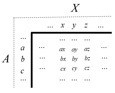
Such conjoint systems are easily visually contemplated if they are thought of as composing a matrix where the rows are values of \(A\), the columns, values of 𝑋, and the cells, values of \(𝑃\). Let \(𝑎\), \(𝑏\), \(𝑐\),… etc. be values of \(𝐴\), \(𝑥\), \(𝑦\), \(𝑧\),… etc. be values of \(𝑋\) and, since \(𝑃 = 𝑓(𝐴, 𝑋)\), the pairs, \(𝑎𝑥\), \(𝑎𝑦\),… , \(𝑐𝑦\), \(c𝑧\),… denote (possibly identical) values of \(P\). Such a matrix is schematically represented by Figure 4.1 to help understand a visual representation of conditions (1) - (3).
4.5.1 Double Cancellation
The double cancellation condition states that if certain pairs of values of \(𝑃\) are ordered by \(≥\), other pairs of specific values will also be ordered. It’s like the transitivity condition that ≥ must satisfy (being a simple order). In the context of conjoint measurement, the transitivity of \(≥\) in \(P\) is a special case of double cancellation.
Double cancellation takes the following form. Let \(𝑎\), \(𝑏\), and \(𝑐\) be any values of \(𝐴\) and \(x\), \(𝑦\), and \(𝑧\) be any values of \(𝑋\), then \(≥\) in \(𝑃\) satisfies double cancellation if and only if
\[ ay \ge bx,\qquad bz \ge cy\quad \Longrightarrow \quad az \ge cx. \]
At first this condition can look abstract. It becomes easier to see when double cancellation is understood as a consequence of the additive case of a non-interactive relation between \(P\), \(A\), and \(X\),
\[ P = A + X. \]
Given this relation,
\[ ay ≥ bx\ \text{if and only if}\ a + y ≥ b + x \] \[ \text{and}\ bz ≥ cy\ \text{if and only if}\ b + z ≥ c + y. \] Adding the two inequalities on the right-hand side we get
\[ a+y+b+z ≥ b+x+c+y \]
and since \(𝑏\) and \(𝑦\) is common on both sides of the inequality, they can be canceled, leaving
\[a + z ≥ c + x\]
which, of course, is true if and only if
\[az ≥ cx\].
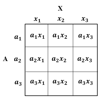
Despite its simplicity, double cancellation is a condition that has considerable power. It strongly restricts the order in \(P\). This can be illustrated in a \(3𝑋3\) matrix. Let \(𝑎1\), \(𝑎2\), and \(𝑎3\) be three values of \(𝐴\) and \(𝑥1\), \(𝑥2\) and \(𝑥3\) be three values of \(𝑋\). The resulting conjoint matrix is illustrated in Figure 4.2.
Now, because \(a\), \(b\), and \(c\) in the double cancellation condition are any values of \(A\), then \(a1\), \(a2\) and \(a3\) can be substituted for them in any of the 3! (= 6) different possible ways. Similarly, \(x1\), \(x2\) and \(x3\) can be replaced by \(x\), \(y\) and \(z\) in 6 different ways. This produces 6 x 6 (= 36) different substitution instances of the double cancellation condition in the 3 x 3 matrix shown above (or in any 3 x 3 conjoint matrix). These 36 different replacement instances are shown in Figure 4.3.
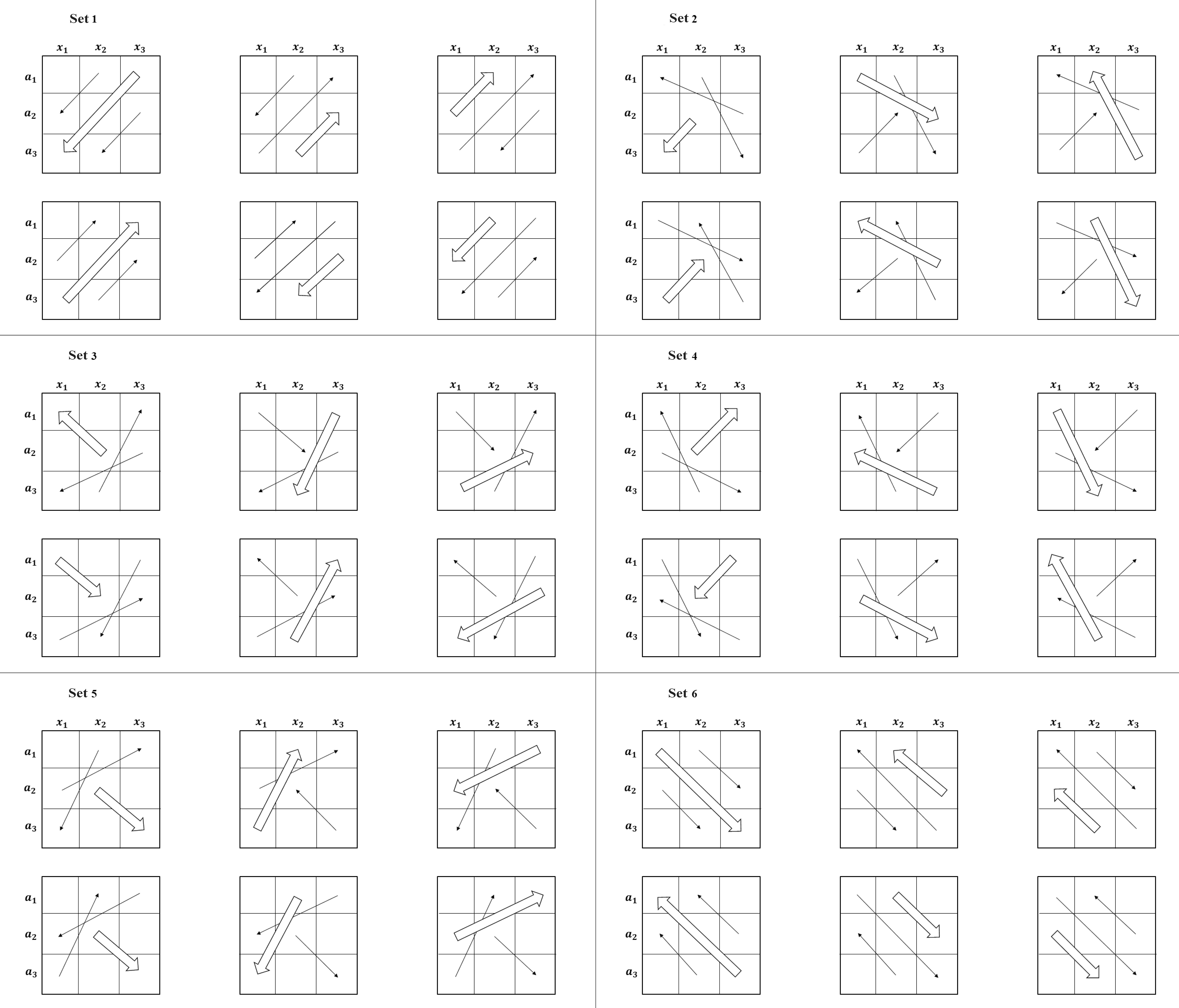
They are not all logically independent of each other. In this, they are in six different sets, each with six. Within each set, the relevant order relations are between the same three values of \(𝑃\) (or matrix cells). Arrows have been used to indicate these relationships (i.e., \(𝑎𝑥 ≥ 𝑏𝑦\) is represented by \(ax\) -> \(by\) , the single-line arrows represent the antecedent orders and double-line arrows represent the consequent order.
Within each set of six, if one of the double cancellation instances is true, they all will be. However, between sets, instances of double cancellation are logically independent of each other. Thus, within any 3 x 3 matrix there are six independent tests of the double cancellation condition, this condition is false if in any of the diagrams shown in the figure above, the antecedent order relations are valid, while the consequent is not; otherwise, they are satisfied. Obviously, satisfying double cancellation (in a conjoint matrix, even a 3 x 3 one) is not a trivial issue and very computationally demanding.
4.5.2 Solvability
The solvability condition requires that the variables \(𝐴\) and \(𝑋\) are complex enough to produce any required value of \(𝑃\). It is formally stated as the following.
The order \(≥\) in 𝑃 satisfies solvability if and only if (i) for any \(𝑎\) and \(b\) in \(𝐴\) and \(x\) in \(𝑋\), there is a value of \(𝑋\) (call it \(𝑦\)) such that \(𝑎𝑥 = 𝑏𝑦\) (i.e., both \(a𝑥 ≥ 𝑏𝑦\) and \(𝑏𝑦 ≥ 𝑎𝑥\)); and (ii) for any \(𝑥\) and \(𝑦\) in \(𝑋\) and \(𝑎\) in \(𝐴\), there is a value of \(𝐴\) (call it \(𝑏\)) such that \(𝑎𝑥 = 𝑏𝑦\). In other words, given any \(𝑎\), \(𝑏\), \(𝑥\), and \(𝑦\), \(𝑦\) exists such that the equation
\[ ax = by \] is solvable.
Thinking in terms of the relationship \(𝑃 = 𝐴 + 𝑋\), solvability implies that the values of \(𝐴\) and \(X\) they are equally spaced (as natural numbers are) or they are dense (as rational numbers are).
4.5.3 Archimedean Condition
As already explained, the Archimedean condition guarantees that no value of a variable quantity is infinitely greater than any other value. Its meaning here is essentially the same, although in this context its expression is a little more complex. Thinking again in terms of \(𝑃 = 𝐴 + 𝑋\), a general idea of its content can be stated as follows. Conjoint measurement allows the quantification of differences between the values of \(A\), between the values of \(𝑋\), and between the values of \(P\). Limiting attention to \(𝐴\), the Archimedean condition means that no difference between any two values of \(𝐴\) is infinitely greater than the difference between any other two values of \(𝐴\).
4.6 The Tale of Taxometric Analysis
The taxometric method introduced by Meehl (1995) is designed to help researchers evaluate whether the latent structure underlying observed data is better characterized as categorical or continuous (Ruscio et al., 2007). In simplified terms, taxometric procedures examine whether the observed pattern is more compatible with a continuous latent dimension or with one or more latent categories (Franco, 2021).
Ruscio & Kaczetow (2009) showed through simulation studies that curve-comparison fit indexes can discriminate dimensional from categorical structures with high accuracy under the conditions they studied. However, a meta-analysis of published taxometric studies found a tendency toward dimensional rather than categorical conclusions (Haslam et al., 2012). Some limitations of taxometrics concern both its statistical interpretation and its relationship with measurement theory. For instance, the covariance structure can create equivalences between certain latent-class and factor representations (Gibson, 1959), which makes taxometric analysis an unfalsifiable method. Moreover, this method has no further developments on current measurement theory, such as testing assumptions of ACM under the psychometric theory.
4.7 Does Rasch Modeling Entail Measurement?
In order to derive a numerical representation of psychological variables, a series of analyses have been developed. Still, conjoint measurement had very little impact on the construction of these psychometric models (Cliff, 1992; Narens & Luce, 1993; Ramsay, 1975, 1991; Schwager, 1991). One model is especially often connected to conjoint measurement: the Rasch model (Rasch, 1960).
| Additive conjoint measurement | Rasch modeling |
|---|---|
| Begins with axioms concerning empirical order and additivity | Begins with a probabilistic response model |
| Asks whether quantitative representation is justified | Asks whether observed responses are compatible with the model |
| Does not require a specific item-response curve | Specifies a particular functional relation between person and item parameters |
| Establishes representational conditions if its axioms hold | Model fit alone does not automatically establish the ACM axioms |
To relate the Rasch model with conjoint measurement, some authors have argued by analogy with physical measurement, an approach criticized by Kyngdon (2008b). For instance, Fischer (1995) reached the conclusion that due to the logarithmic transformations yielding additive connections between derived measurements in physics, it logically follows that the constructs of individual ability and item complexity possess adequate complexity to support representation theorems extending to real numbers, which are essentially unique barring linear adjustments. In essence, individual ability and item difficulty are deemed to exhibit additive structures solely based on altering the relationship between these constructs. This relationship, however, is held by analogy to derived measurement through the notion of specific objectivity (Kyngdon, 2008b). To assert that an additive interval measurement of a person’s ability and item difficulty is given by the Rasch model (Rasch, 1960), it’s required that the underlying assumption is true: test performance is a multiplicative conjoint structure comprising of a person’s ability and the item difficulty. Nonetheless, this has not been proven elsewhere.
Much of the literature connecting Rasch modeling and conjoint measurement treats the Rasch model as a probabilistic realization of conjoint measurement (Borsboom & Mellenbergh, 2004; Karabatsos, 2001; Kline, 1998; see also Kyngdon, 2008a). On this view, data fitting the Rasch model may support interval scaling. However, this claim is controversial. Michell (2008) emphasizes that conjoint measurement is formulated in terms of ordinal and equivalence relations required for quantification, whereas the Rasch model starts from a probabilistic response function. Therefore, the connection between the two frameworks requires argument rather than being a straightforward mathematical equivalence (Kyngdon, 2008a). The difference between Rasch and the theory of conjoint measurement is mathematically clear. The theory of conjoint measurement proposes axioms for order and additivity (Luce & Tukey, 1964), whereas the Rasch model primarily imposes a probabilistic ordering structure on persons and items (Borsboom & Zand Scholten, 2008).
In standard research practice, when a person runs a Rasch model, they supposedly check for the consistency between the data and model with measurement axioms using fit statistics (Karabatsos, 2001). However, even if we assume that Rasch is testing those axioms, the test using fit statistics is not straightforward, since the specification of additive conjoint measurement under the Rasch model is data-dependent. This is because the Item Response Function is estimated directly from data, and data contains random or systematic noise. This problem is illustrated by Nickerson & McClelland (1984) and Karabatsos (2001): a numerical or probabilistic model can show very good fit even when relevant conjoint-measurement restrictions are violated.
4.7.1 Representationally Adequate Item Response Theory Models
Scheiblechner (1995) developed the Isotonic Ordinal Probabilistic Model (ISOP), with later corrections and clarifications provided by Scheiblechner (1998), partly to address limitations in more restrictive parametric measurement models. ISOP operates on the premise that in Experimental or Testing Psychology, it is common to hypothesize an ordinal variable before experiments, allowing the ranking of observed reactions. This model fits by testing axioms I and II from additive conjoint measurement theory and is often referred to as a probabilistic approach closely related to nonparametric item-response models and Mokken scaling (Molenaar, 1991).
Unlike parametric latent trait models, ISOP is nonparametric, meaning it doesn’t rely on a specific parametric family, functional curve form, or prior distribution of latent ability. It is based on axiomatic principles, with independent and separately testable axioms, offering nonparametric statistical tests for various unidimensional models. This structure enables ISOP to distinguish between poor fit caused by latent trait multidimensionality and poor parameterization.
The ISOP model provides a foundational framework in measurement theory, emphasizing ordinal unidimensionality and offering algorithms and technologies for test development. It assumes that responses are generated by the interaction of individuals and items, producing a common ordinal scale, but the effects are not additive. Scheiblechner (1999) extended ISOP by incorporating the cancellation axiom (axiom III), resulting in the Additive Conjoint Isotonic Probabilistic Model (ADISOP). This extension allows for the creation of two ordered metric scales with a shared unit for both subjects and items, enabling an additive representation of latent variables that interact to produce the observed orders.
Although ADISOP shares similarities with the Rasch model, it does not prescribe a specific item response function. Scheiblechner (1999) suggests that comparing ISOP, ADISOP, and the Rasch model can help assess the measurement level of latent variables. These models form a hierarchy, transitioning from ordinal to interval measures (if ADISOP fits better than ISOP) and from interval measures with uncertainty to those with a strong functional form (if the Rasch model fits better than ADISOP).
| Model | Main emphasis | Measurement interpretation |
|---|---|---|
| ISOP | Ordinal probabilistic structure | Common ordinal ordering |
| ADISOP | Adds cancellation/additive requirements | Supports an additive representation when its axioms hold |
| Rasch | Adds a specific probabilistic functional form | Stronger parametric structure if the model is appropriate |
4.8 The Direct Test of Conjoint Measurement Axioms
A Bayesian approach initiated by Karabatsos (2001) and further developed by Domingue (2014) makes it possible to test ACM axioms. Suppose there’s a unidimensional latent variable, which has a function linking the persons’ responses to a set of items. Consider that \(P\) is an \(I x J\) matrix that contains the true response probabilities for this set of items. Each cell in the conjoint matrix \(P^{MLE}\), with dimensions \(I x J\), contains the percentage of respondents with a certain ability who answered the appropriate item correctly.
In order to determine whether the axioms are true for \(P\), the order restrictions from the cancellation axioms are imposed stochastically via a Metropolis–Hastings sampling procedure (Hastings, 1970; Metropolis et al., 1953). Domingue (2014) conducted simulation studies to test the new approach, and the evidence suggests that this approach can discriminate between data generated via the Rasch model and the 3PL model. This is expected, given that the 3PL item response model does not follow the axioms of additive conjoint measurement.
There is an R package called ConjointChecks, associated with this line of work (Domingue, 2014), that can be used to test cancellation assumptions from additive conjoint measurement. The package can be installed from GitHub as follows.
The important point is not the software itself. The conceptual advance is that measurement axioms are being treated as empirical restrictions that can be confronted with data, rather than assumptions silently accepted because a familiar psychometric model was fitted.
4.9 From Measurement Theory to Model Comparison: A Recent Approach
The previous sections show why interval-level measurement should not be treated as an automatic consequence of assigning numbers to responses or fitting a familiar psychometric model. A practical difficulty remains, however: how can we compare an ordinal representation with stronger additive representations using ordinary response data?
In a recent study, Degobi et al. (2026) proposed a model-comparison framework designed to make this assumption empirically contestable. Instead of beginning with models that all presuppose an interval latent metric, the approach compares three models that represent increasingly strong measurement claims:
| Model | What it requires | Measurement-level interpretation |
|---|---|---|
| ISOP | Invariant ordering of persons and items | A common ordinal representation is sufficient |
| ADISOP | ISOP restrictions plus an additive/cancellation structure | Evidence is consistent with an interval-level additive representation, without fixing the response-function shape |
| Rasch | Additivity plus a specific logistic response function | Evidence favors the stronger additive + logistic representation |
This hierarchy separates two questions that are often combined in standard IRT applications. First, is the ordinal structure sufficient, or does the data support an additive person–item representation? Second, if additivity is supported, is there also evidence for the particular logistic functional form imposed by the Rasch model?
The question is no longer simply “Does the Rasch model fit?” Instead, the level of measurement becomes part of the model-comparison problem: does the data support only an ordinal representation, an additive representation with an unspecified monotonic response function, or the more restrictive Rasch representation? (Degobi et al., 2026)
4.9.1 Comparing models with effective degrees of freedom
A complication is that ISOP and ADISOP are isotonic models. Their complexity is not conveniently represented by a simple count of free parameters. Degobi et al. (2026) therefore estimated effective degrees of freedom (EDF) using respondent-level bootstrap samples and used this quantity as the complexity penalty in several information criteria.
Let \(D\) be the deviance of a model fitted to the original data and \(\overline{D}_{boot}\) the mean deviance across bootstrap refits. The bootstrap estimate used in the study is
\[ EDF = D - \overline{D}_{boot}. \]
The resulting information criteria are
\[ AIC^* = D + 2(EDF), \]
\[ BIC^* = D + \log(N)(EDF), \]
and
\[ HQC^* = D + 2(EDF)\log\{\log(N)\}. \]
The study also examined a bootstrap analogue of DIC using the variability of bootstrap deviances as a complexity term. This last criterion was treated more cautiously because it is not conventional posterior DIC and showed computational instability in some simulation conditions (Degobi et al., 2026).
4.9.2 What did the study find?
The simulation deliberately generated data from an additive Rasch structure. It crossed five test lengths (10, 20, 30, 50, and 100 items), three sample sizes (100, 500, and 1,000), and three response formats (2, 5, and 7 categories), yielding 45 conditions. One hundred independent datasets were generated in each condition.
The main result was not that a single design feature reliably determined which model would be selected. Model selection depended on the joint combination of test length, sample size, response format, and information criterion. AIC, BIC, and HQC frequently preferred ADISOP for polytomous data, meaning that they often recovered the additive measurement structure without requiring the stronger Rasch logistic form. For some longer dichotomous tests, however, these criteria shifted toward ISOP even though the data had been generated from a Rasch model. The bootstrap DIC often behaved differently from the other criteria (Degobi et al., 2026).
The empirical illustration used 45 dichotomously scored Language items from the Brazilian National High School Examination (ENEM). With a random sample of 500 examinees, AIC and HQC favored ISOP, whereas BIC and the bootstrap DIC favored Rasch. With all 4,639 complete cases, AIC, BIC, and HQC favored ISOP, while the bootstrap DIC continued to favor Rasch (Degobi et al., 2026).
The paper does not recommend counting how many criteria choose each model and declaring the majority the winner. The simulation showed that the criteria can behave differently even when the true generating structure is known. Agreement across criteria is stronger evidence; disagreement is evidence that the measurement-level conclusion is unstable under the current procedure.
The proposal therefore should not be interpreted as a definitive test that can prove that a psychological attribute is quantitative. Its more modest contribution is to replace an assumption that is usually left untested with an explicit comparison among weaker and stronger measurement representations. The paper also emphasizes the need for simulation-based calibration under design conditions similar to the application of interest before making high-stakes claims about measurement level (Degobi et al., 2026).
4.10 Worked Example: Measurement Level of the BFI Agreeableness Items
We can apply the same logic to a small psychological example using the first five variables of the psych::bfi dataset:
These are the five Agreeableness items (A1 to A5). Because A1 is negatively keyed relative to the other Agreeableness items, we reverse it before fitting a common person–item ordering. The response scale runs from 1 to 6, so the reverse-scoring transformation is \(7-A1\).
This example is intended to demonstrate the workflow, not to establish that Agreeableness is truly ordinal or interval-scaled. With only five items, the design differs substantially from many conditions studied by Degobi et al. (2026). Any substantive conclusion should therefore be supported by additional validation work and, ideally, simulations calibrated to this particular design.
4.10.1 1. Prepare the data
Show data preparation
# install.packages(c("psych", "sirt"))

Data <- psych::bfi[, c(1:5)]

# A1 is negatively keyed relative to the other Agreeableness items.
Data$A1 <- 7 - Data$A1

# The ISOP/ADISOP analysis below uses complete response patterns.
Data <- Data[complete.cases(Data), ]

# Convert to a numeric matrix.
Data <- as.matrix(Data)
storage.mode(Data) <- "numeric"

dim(Data)
head(Data)
apply(Data, 2, table)
Before proceeding, it is useful to inspect the response distributions. Very sparse categories, unusual response patterns, or coding errors can affect the fitted order restrictions.
4.10.2 2. Fit ISOP, ADISOP, and Rasch models
The sirt::isop.poly() function returns log-likelihoods for the saturated, ISOP, ADISOP, and Rasch representations. The wrapper below extracts the values needed for the model-comparison procedure.
The four returned values correspond, in order, to the saturated model, ISOP, ADISOP, and Rasch model.
4.10.3 3. Estimate model complexity by bootstrap
The paper used 1,000 respondent-level bootstrap replications. Because this can take some time, the code below keeps the number of replications in a single object so it can easily be reduced while learning the procedure.
Show bootstrap code
set.seed(2026)

B <- 1000L

boot_worker_isop <- function(k, data) {

  data_boot <- data[
    sample.int(nrow(data), nrow(data), replace = TRUE),
    ,
    drop = FALSE
  ]

  isop_wrapper(data_boot)
}

n_cores <- max(1L, parallel::detectCores() - 1L)
cl <- parallel::makeCluster(n_cores)

parallel::clusterEvalQ(cl, {
  library(sirt)
})

parallel::clusterExport(
  cl,
  c("isop_wrapper", "boot_worker_isop"),
  envir = environment()
)

bs_ll <- tryCatch(
  parallel::parSapply(
    cl = cl,
    X = seq_len(B),
    FUN = boot_worker_isop,
    data = Data
  ),
  finally = parallel::stopCluster(cl)
)When first trying the code, set B <- 100 or B <- 200. For a substantive analysis, increase the number of bootstrap replications and examine whether the resulting EDF and model-selection conclusions are stable. The manuscript used 1,000 bootstrap replications.
4.10.4 4. Calculate the information criteria
We now transform log-likelihoods to deviances, estimate effective degrees of freedom, and calculate AIC, BIC, HQC, and the bootstrap analogue of DIC using the same formulas as the empirical example in Degobi et al. (2026).
Show information-criterion calculations
# Bootstrap deviances
bs_dev <- -2 * bs_ll

# Original deviances
Dev <- -2 * ll_orig

# Mean bootstrap deviance
Dbar <- rowMeans(bs_dev, na.rm = TRUE)

# Effective degrees of freedom
edf <- Dev - Dbar

# Variance-based complexity term for bootstrap DIC
pD <- apply(bs_dev, 1, var, na.rm = TRUE) / 2

# Information criteria
AIC <- Dev + 2 * edf
BIC <- Dev + log(nrow(Data)) * edf
HQC <- Dev + 2 * edf * log(log(nrow(Data)))
DIC <- Dbar + pD

Results <- round(
  t(
    data.frame(
      Dev = Dev,
      Dbar = Dbar,
      edf = edf,
      pD = pD,
      AIC = AIC,
      BIC = BIC,
      HQC = HQC,
      DIC = DIC
    )
  ),
  3
)

colnames(Results) <- c(
  "Saturated",
  "ISOP",
  "ADISOP",
  "Rasch"
)

Results
The smallest information-criterion value indicates the preferred model for that criterion. We can summarize those selections directly:
Show model-selection summary
criteria <- c("AIC", "BIC", "HQC", "DIC")
candidate_models <- c("ISOP", "ADISOP", "Rasch")

selected_model <- vapply(
  criteria,
  function(criterion) {

    values <- Results[
      criterion,
      candidate_models
    ]

    names(which.min(values))
  },
  character(1)
)

data.frame(
  Criterion = criteria,
  Selected_Model = selected_model,
  row.names = NULL
)
4.10.5 5. Interpret the result as a comparison of measurement claims
The result should be interpreted according to the restrictions encoded by the competing models:
- ISOP selected: the criterion prefers the weaker common ordinal representation over the additive alternatives.
- ADISOP selected: the criterion provides evidence consistent with an additive representation, but the additional Rasch logistic restriction is not needed.
- Rasch selected: the criterion favors the additive representation together with the Rasch logistic functional form.
- Criteria disagree: the data do not yield a stable measurement-level conclusion under this procedure.
Notice that none of these outcomes should be translated into statements such as “Agreeableness has been proven to be interval-scaled.” Model selection is always relative to the candidate representations and their empirical restrictions. The main advantage of the analysis is that the ordinal-versus-additive distinction becomes something we can examine rather than something we silently assume (Degobi et al., 2026).
4.11 Concluding Remarks
The central argument of this chapter is simple, even though the theory is not: using numbers is not sufficient to establish measurement. A measurement claim requires a defensible relationship between the structure of an empirical attribute and the numerical structure used to represent it.
This is why the distinction between numerical coding and measurement is so important in psychology. Psychometric models can be extremely useful, but their statistical structure should not automatically be treated as proof that the psychological attribute itself is quantitative. Additive conjoint measurement provides one framework for making these assumptions explicit through order, cancellation, solvability, and Archimedean conditions.
The debates surrounding taxometrics, Rasch modeling, ISOP, ADISOP, and direct tests of conjoint-measurement axioms all return to the same question: what empirical evidence justifies the numerical interpretation we give to psychological scores? Keeping this question visible helps connect measurement theory with the broader concerns about validity developed earlier in the book and with the psychometric models introduced in the chapters that follow.