3 Constructs and Latent Variables in Psychometrics
Psychometrics is not only a collection of statistical techniques. It is also a framework for connecting psychological concepts to observable data. This chapter focuses on one of the most important ideas behind modern psychometrics: the reflective latent variable.
NoteChapter map
By the end of this chapter, you should be able to distinguish a construct from a reflective latent variable and an indicator, explain why PCA is not a latent-variable model, compare reflective, formative, network, and latent-class representations, and understand why some reflective models imply testable constraints such as vanishing tetrads.
3.1 Why a Reflective Latent Variables Matter
Psychometrics focuses on the measurement and quantitative representation of psychological attributes, behaviors, performance, and emotions. Measurement problems are therefore not peripheral to psychological science: if the link between a theoretical attribute and the observed scores is poorly specified, substantive conclusions can also become uncertain (Borsboom et al., 2004; Cronbach & Meehl, 1955; Messick, 1989).
Modern psychometric models provide a language for making these links more explicit. They force us to ask what an observed score represents, why indicators covary, and which assumptions are required to interpret that covariation psychologically (Borsboom, 2006). This is one reason psychometric modeling is more than a technical step performed after data collection: the measurement model is part of the substantive theory.
TipA recurring principle in this book
A statistical model can fit the data well and still be a poor representation of the phenomenon. Model choice should follow from the substantive theory and the intended interpretation of the scores—not from fit indices alone.
3.2 Two Common Conceptual Mistakes
3.2.1 PCA is not a Reflective latent-variable model
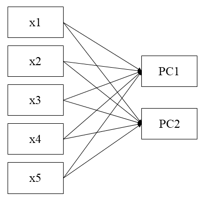
A common source of confusion is the use of principal component analysis (PCA) when the research question concerns latent variables. PCA is a data-reduction method: components are weighted combinations of observed variables. It does not posit an unobserved common cause that generates the indicators (Bartholomew, 2004).
This does not make PCA a bad method. The problem arises when a principal component is interpreted as though it were automatically evidence for a reflective latent psychological attribute, instead of a formative model. If the scientific claim is about a latent variable, the statistical model should contain a latent-variable structure that corresponds to that claim.
3.2.2 Observed group differences are not automatically construct differences
A second mistake occurs when observed-score differences between groups are interpreted directly as differences in the psychological attribute. Such comparisons require assumptions about measurement invariance: the measurement model should operate comparably across the groups being compared (Mellenbergh, 1989; Meredith, 1993; Millsap & Everson, 1993).
Without this evidence, a group difference in an observed score may reflect a difference in the target attribute, a difference in how the instrument functions across groups, or some combination of the two. This issue is developed in detail in the later chapter on measurement invariance.
3.3 Why This Is Difficult in Practice
Psychometric models often make assumptions that are easy to overlook when only total scores are analyzed. Questions about dimensionality, measurement invariance, local independence, and the causal interpretation of latent variables can quickly become questions about the theory of the phenomenon itself (Borsboom, 2006).
This is demanding because statistical modeling cannot decide these questions on its own. Researchers need a defensible construct definition, a plausible account of why indicators should relate to one another, and empirical evidence that is capable of challenging those assumptions. The apparent complexity of psychometrics is therefore partly a consequence of taking measurement claims seriously.
3.4 Constructs, Referents, and Latent Variables
Scientific concepts help researchers organize and communicate about phenomena. Their meanings depend on rules of use, and unclear or unstable terminology can make scientific results difficult to compare or replicate (Maraun & Peters, 2005; Schmalz et al., 2024). Psychology uses many such concepts—stress, intelligence, self-esteem, depression, well-being, and countless others—to organize observations and theories.
The history of psychological measurement reflects an effort to represent these attributes quantitatively (Michell, 2014). Yet this requires care because psychological constructs are usually not directly observable in the way that physical length can be read from a ruler (Michell, 2001; Trendler, 2013).
Uher (2022) describes a construct as a conceptual system that groups referents considered meaningfully related for a particular purpose. In this sense, a construct is not simply one questionnaire item or one observed behavior. Following the tradition of Cronbach & Meehl (1955), constructs are useful precisely because they organize multiple observable referents that cannot all be reduced to one direct observation.
ImportantThree things that should not be conflated
| Concept | What it is | Example |
|---|---|---|
| Construct | A theoretical/conceptual system used to organize phenomena | Depression |
| Indicator | An observed variable used to obtain information relevant to the construct | Response to “I felt sad most of the day” |
| Latent variable | An unobserved variable in a statistical model | A continuous common factor fitted to depression items |
The three can be related, but they are not interchangeable.
Constructs are conceptual tools rather than physical objects (Uher, 2023). Confusing the construct with the phenomenon it is intended to organize has been called construct–referent conflation (Maraun & Gabriel, 2013). A related problem occurs when variables in a data set are discussed as though they were the phenomena themselves; Uher (2021) describes this as a form of variable–referent conflation.
A latent variable is one statistical tool—among several possible approaches—for representing relationships among observed indicators. The common-factor tradition can be traced to Spearman (1904), and later latent-variable models formalized relationships between theoretical attributes and their observed measures (Bollen, 1989; Edwards & Bagozzi, 2000). Indicators may be questionnaire items, interview ratings, behavioral observations, performance measures, or other observed variables (DeVellis & Thorpe, 2021; Lord & Novick, 1968).
3.5 Ways to Represent a Construct
The way a construct is represented statistically should follow from a claim about why the indicators are related. Four broad representations are useful to distinguish.
| Representation | Basic idea | Direction/structure | Typical methods |
|---|---|---|---|
| Reflective/common factor | A latent variable accounts for covariation among indicators | Latent variable → indicators | EFA, CFA, many IRT models |
| Composite/formative | Indicators jointly define or form a composite | Indicators → composite | Weighted composites, some SEM formulations |
| Network | Indicators can influence or interact with one another directly | Indicator ↔︎ indicator | Psychometric network models |
| Latent class/profile | An unobserved categorical grouping accounts for response patterns | Latent class → response distribution | LCA, LPA, mixture models |
3.5.1 Reflective common-factor models
In a common-factor model, covariation among observed variables is explained by one or more latent factors. In its simplest form, the model assumes that once the common factor is taken into account, the indicators are locally independent. This is a strong substantive assumption, not merely a convenient statistical convention (Bollen, 1989).
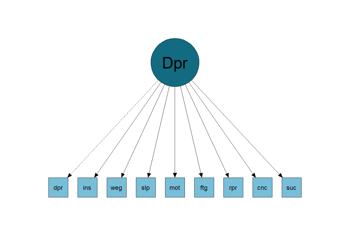
Consider symptoms of major depression. A reflective factor model might represent depressed mood, sleep disturbance, fatigue, concentration problems, and other symptoms as indicators of a common latent variable. In this representation, variation in the latent factor accounts for the associations among the symptoms.
3.5.2 Network representations
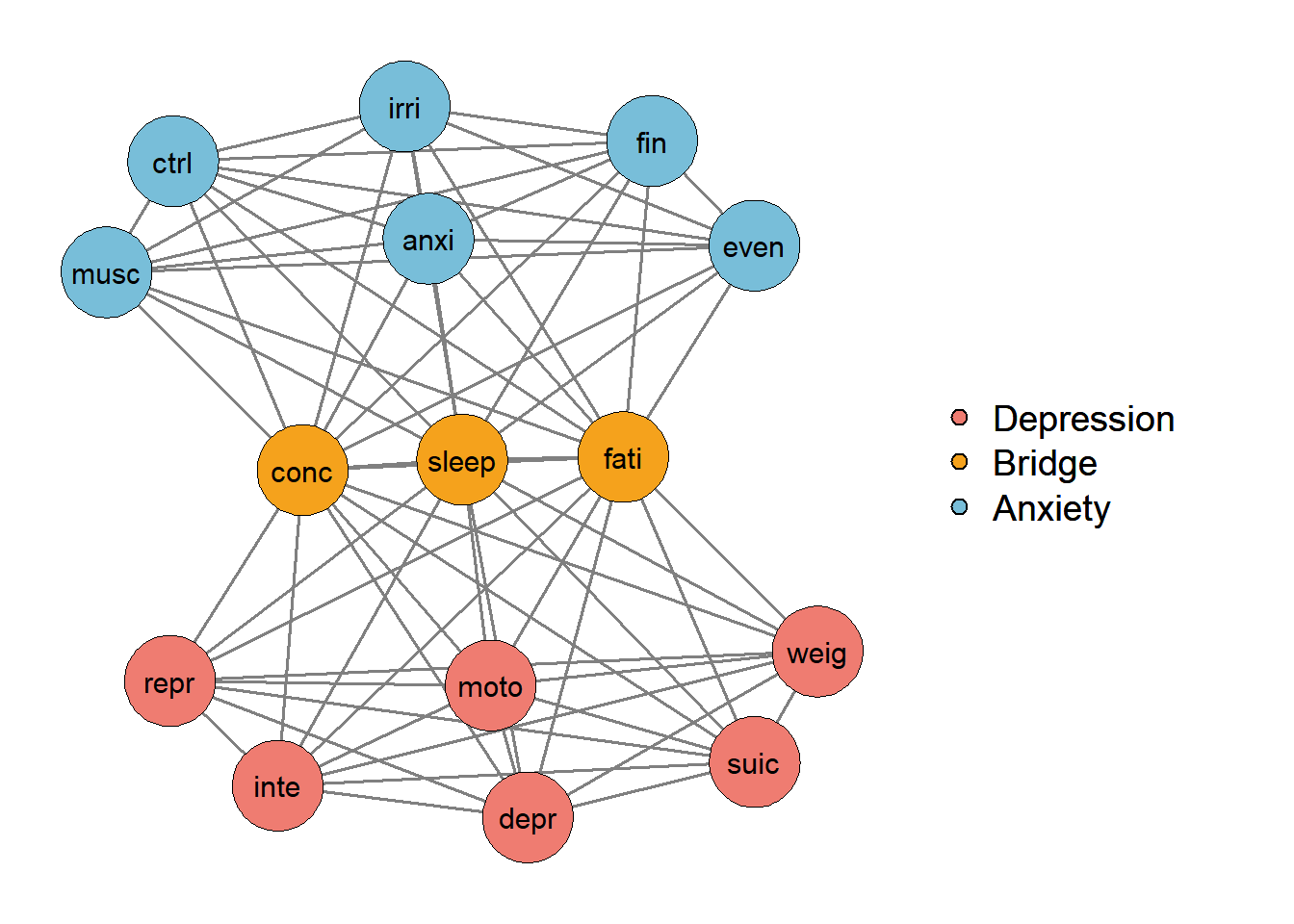
A different theory is possible. Sleep problems may contribute to fatigue, fatigue may contribute to concentration problems, and these symptoms may reinforce one another. In this account, at least part of the covariation is generated by relationships among the indicators themselves, rather than solely by a common latent cause. This is the basic motivation for network representations of psychopathology (Borsboom & Cramer, 2013).
TipTheory first
The choice between a factor model and a network model is not settled by asking which graph looks better or which model produces more attractive fit statistics. The models make different claims about why variables covary. Those claims should be motivated theoretically and then exposed to empirical tests.
3.5.3 Composite and formative representations
A composite or formative representation reverses the usual reflective logic: the indicators jointly define the composite. Socioeconomic status is a common example because income, education, and occupational or housing characteristics can be combined to define an index. Changing an indicator can change the composite rather than being interpreted as an effect of a single underlying common cause (Edwards & Bagozzi, 2000).
PCA can also construct weighted composites, but PCA and formative measurement should not be treated as synonyms. PCA is an algebraic method for summarizing variance; a formative measurement interpretation adds a substantive claim about what the composite represents.
3.5.4 Latent classes and profiles
Latent class analysis (LCA) and latent profile analysis (LPA) represent unobserved heterogeneity categorically rather than continuously. Instead of locating people along a continuous factor, these models describe unobserved classes or profiles that differ in their response patterns (Muthén & Muthén, 2000; Oberski, 2016). Mixture models can also connect categorical and continuous representations (Loken & Molenaar, 2008). The distinction between continuous and categorical numerical representations is developed further in Chapter 4.
3.6 Reflective Models and Causal Interpretation
Reflective measurement is often written as though the latent variable produces variation in its indicators. For example, if self-esteem is represented reflectively, differences in the latent variable are assumed to generate systematic differences in item responses. This causal reading is explicit in some psychometric traditions and implicit in many others (Bollen, 1989; Bork et al., 2017).

The reflective logic appears in many familiar models, including the common-factor model, many item response theory models, latent growth models, and other latent-variable approaches (Hambleton et al., 1991; Lord & Novick, 1968; Meredith & Tisak, 1990). However, it is important to distinguish using causal language from establishing a causal relation. The presence of an arrow in a path diagram does not by itself demonstrate causality (Pearl, 2009).
Some authors instead favor a descriptivist interpretation in which the latent variable is a parsimonious statistical representation rather than a real common cause (Bork et al., 2017; Jonas & Markon, 2016). The difference matters because a causal common-factor interpretation implies more than a good-fitting covariance model: it implies that the observed associations arise in a way compatible with the proposed causal structure.
ImportantLocal independence is a substantive claim
In a simple reflective model, indicators are expected to become independent after conditioning on the common latent variable. If two items still influence one another directly—for example, sleep problems causing fatigue—then the local-independence assumption can fail even when a one-factor model appears superficially plausible.
3.7 Vanishing Tetrads: A Testable Implication
One way to examine implications of a linear common-cause model is through tetrad constraints. Spearman’s early work showed that a single common factor imposes restrictions on the covariance matrix (Spearman, 1904). These ideas were later developed in structural equation modeling and confirmatory tetrad analysis (Bollen, 1989; Bollen & Ting, 1993).
A tetrad is a difference between two products of covariances. For four observed variables, one example is
\[ \tau_{1234} = \sigma_{12}\sigma_{34} - \sigma_{13}\sigma_{24}. \]
A tetrad vanishes when this difference is zero in the population. In a simple one-factor model with four indicators and independent residuals, several such constraints are implied. They are useful because they are observable consequences of the model rather than statements about an unobserved factor alone.
3.7.1 Treks and covariance constraints
A convenient way to understand these constraints is through a directed graph. A directed path from \(u\) to \(v\) is a sequence of arrows all pointing toward \(v\). A trek is a path or pair of directed paths that connects two variables without colliding arrowheads. Under linear models, trek rules can be used to derive the covariance constraints implied by a graph (Glymour et al., 2014; Glymour & Scheines, 1986).
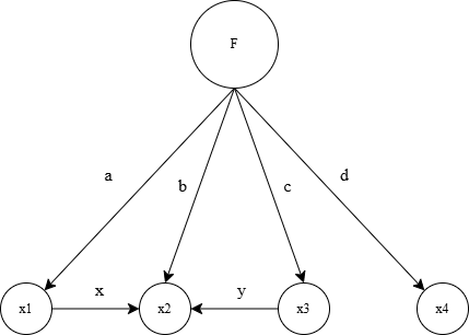
Each valid trek contributes to the covariance between two variables. In a standardized linear model, the contribution of a trek is obtained from the product of the coefficients along that trek; the covariance is the sum of the contributions from the available treks.
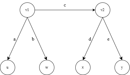
For the illustrated model, suppose the standardized correlations implied by the paths are
\[ \begin{aligned} \rho_{uw} &= ab, & \rho_{ux} &= acd, & \rho_{uy} &= ace,\\ \rho_{xy} &= de, & \rho_{wy} &= bce, & \rho_{wx} &= bcd. \end{aligned} \]
Then the model implies
\[ \rho_{ux}\rho_{wy}=\rho_{uy}\rho_{wx}. \]
Adding a direct path that changes one side of this relation can destroy the equality. The tetrad therefore acts as a testable implication of the specified graph.
3.7.2 Tetrads in a one-factor model
Consider a one-factor model with four standardized indicators. If the factor loadings are \(\lambda_1,\lambda_2,\lambda_3,\lambda_4\) and the residuals are mutually independent, then
\[ \rho_{12}=\lambda_1\lambda_2, \qquad \rho_{34}=\lambda_3\lambda_4, \]
and likewise for the other pairs. Consequently,
\[ \rho_{12}\rho_{34} = \rho_{13}\rho_{24} = \rho_{14}\rho_{23}. \]
The important idea is not that a vanishing tetrad proves that a latent variable causes the indicators. Rather, the proposed model implies constraints on observable covariances. If the population covariance matrix violates those constraints, the simple model cannot be exactly correct. If the constraints are compatible with the data, the model remains plausible under the assumptions used to derive them (Bollen & Ting, 1993; Glymour et al., 2014).
WarningCompatibility is not proof of causality
Vanishing tetrads can rule out some covariance structures, but they do not uniquely establish a causal common factor. Different causal models can sometimes imply the same observational constraints. Tetrads should therefore be interpreted as one source of evidence about model structure, not as a standalone causal proof.
Other testable constraints can involve zero covariances, equal covariances, zero partial correlations, equality constraints, or higher-order polynomial relations. Tetrads are especially important in multiple-indicator models because they arise naturally from simple common-factor structures (Glymour & Scheines, 1986). Related approaches to assessing the causal implications of factor models are discussed by Franco et al. (2023).
3.7.3 Vanishing Tetrads in R
The following example uses four Openness items from the bfi data set in the psych package. The goal is not to prove that Openness is a causal latent variable. Instead, we ask whether these observed variables are compatible with the tetrad constraints implied by a simple common-factor structure.
The CauseAndCorrelation package contains a vanishing.tetrads() function. If the package can be installed in your R environment, the workflow is:
Because package availability can change over time, the function used in this example is included below so that the logic of the tutorial remains reproducible.
Show vanishing.tetrads() function
vanishing.tetrads<-function (dat, sig = 0.05)
{
    get.3.equations <- function(tet.vector) {
        mat <- matrix(NA, ncol = 8, nrow = 3)
        mat[1, ] <- cbind(tet.vector[1], tet.vector[2], tet.vector[3],
            tet.vector[4], tet.vector[1], tet.vector[4], tet.vector[2],
            tet.vector[3])
        mat[2, ] <- cbind(tet.vector[1], tet.vector[3], tet.vector[2],
            tet.vector[4], tet.vector[1], tet.vector[4], tet.vector[2],
            tet.vector[3])
        mat[3, ] <- cbind(tet.vector[1], tet.vector[3], tet.vector[2],
            tet.vector[4], tet.vector[1], tet.vector[2], tet.vector[3],
            tet.vector[4])
        mat
    }
    test.stat <- function(dat, triplet) {
        t.vars <- sort(triplet[1:4])
        r <- var(dat, na.rm = T)
        tao <- r[triplet[1], triplet[2]] * r[triplet[3], triplet[4]] -
            r[triplet[5], triplet[6]] * r[triplet[7], triplet[8]]
        D13 <- det(r[c(triplet[1], triplet[3]), c(triplet[1],
            triplet[3])])
        D24 <- det(r[c(triplet[2], triplet[4]), c(triplet[2],
            triplet[4])])
        D <- det(r[triplet[1:4], triplet[1:4]])
        N <- dim(dat)[1]
        tao.var <- (D13 * D24 * (N + 1)/(N - 1) - D) * (1/(N -
            2))
        if (tao.var <= 0) {
            cat("triplet: ", triplet, "\n")
            cat("variance of tao is ", tao.var, "\n")
            cat("tao.var<=0. D=", D, "D13=", D13, "D24=", D24,
                "\n")
            stop()
        }
        z <- tao/sqrt(tao.var)
        list(triplet = triplet, VCV = r, tao = tao, tao.var = tao.var,
            z = z, prob = 2 * (1 - pnorm(abs(z))))
    }
    get.choke.points <- function(vec) {
        tetrad <- matrix(vec, ncol = 2, byrow = T)
        all.comb <- cbind(c(vec[1], vec[1], vec[1], vec[2], vec[2],
            vec[3]), c(vec[2], vec[3], vec[4], vec[3], vec[4],
            vec[4]))
        chokes <- rep(T, 6)
        for (j in 1:4) {
            for (i in 1:6) {
                if (sum(tetrad[j, ] == all.comb[i, c(1, 2)]) ==
                  2)
                  chokes[i] <- F
                if (sum(tetrad[j, ] == all.comb[i, c(2, 1)]) ==
                  2)
                  chokes[i] <- F
            }
        }
        list(tetrad = tetrad, all.comb = all.comb, choke.points = all.comb[chokes,
            ])
    }
    nvars <- dim(dat)[2]
    tetrad.quadriplets <- combn(1:nvars, 4)
    ntetrads <- dim(tetrad.quadriplets)[2]
    z <- prob <- rep(NA, ntetrads * 3)
    count <- 0
    for (i in 1:ntetrads) {
        triplets <- get.3.equations(tetrad.quadriplets[, i])
        for (j in 1:3) {
            count <- count + 1
            temp <- test.stat(dat, triplets[j, ])
            z[count] <- temp$z
            prob[count] <- temp$prob
            if (prob[count] <= sig)
                cat("triplet:", triplets[j, ], " does not vanish (p=",
                  prob[count], ") \n\n")
            if (prob[count] > sig) {
                chokes <- get.choke.points(triplets[j, ])
                cat("triplet:", triplets[j, ], "  vanishes (p=",
                  prob[count], ") \n")
                cat("If there is a saturated dependency graph for the four variables (via EPA):",
                  triplets[j, 1], triplets[j, 2], triplets[j,
                    3], triplets[j, 4], "\n")
                cat("then there is at least one latent common cause of either (",
                  chokes$choke.points[1, 1], ",", chokes$choke.points[1,
                    2], ") and/or of (", chokes$choke.points[2,
                    1], ",", chokes$choke.points[2, 2], ")\n\n")
            }
        }
    }
}
The function evaluates each unique set of four variables and tests the corresponding tetrad equations. Here we use four Openness items:
       O1              O2              O3              O4
 Min.   :1.000   Min.   :1.000   Min.   :1.000   Min.   :1.000
 1st Qu.:4.000   1st Qu.:1.000   1st Qu.:4.000   1st Qu.:4.000
 Median :5.000   Median :2.000   Median :5.000   Median :5.000
 Mean   :4.816   Mean   :2.713   Mean   :4.438   Mean   :4.892
 3rd Qu.:6.000   3rd Qu.:4.000   3rd Qu.:5.000   3rd Qu.:6.000
 Max.   :6.000   Max.   :6.000   Max.   :6.000   Max.   :6.000
 NAs    :22                      NAs    :28      NAs    :14
Now evaluate the tetrads:
triplet: 1 2 3 4 1 4 2 3   vanishes (p= 0.4600686 )
If there is a saturated dependency graph for the four variables (via EPA): 1 2 3 4
then there is at least one latent common cause of either ( 1 , 3 ) and/or of ( 2 , 4 )

triplet: 1 3 2 4 1 4 2 3  does not vanish (p= 0.03361732 )

triplet: 1 3 2 4 1 2 3 4   vanishes (p= 0.1174989 )
If there is a saturated dependency graph for the four variables (via EPA): 1 3 2 4
then there is at least one latent common cause of either ( 1 , 4 ) and/or of ( 3 , 2 )
If at least one implied tetrad is statistically inconsistent with zero, the observed covariance structure is not fully consistent with all of the constraints of that simple factor representation. The reverse conclusion should be more cautious: failure to reject a tetrad does not prove that a common latent cause exists.
3.8 Concluding Remarks
Latent variables are powerful because they allow researchers to connect unobserved theoretical attributes to patterns in observed data. But that power comes from assumptions. A common-factor model, a network model, a composite, and a latent-class model can all summarize the same broad set of indicators while making very different claims about why those indicators are related.
The central lesson is therefore to keep constructs, observed indicators, and statistical latent variables conceptually distinct. The model should be selected because its assumptions are defensible for the phenomenon and the intended interpretation—not simply because it is a familiar psychometric routine.
In the next chapters, exploratory and confirmatory factor analysis will provide practical tools for studying latent structure. The conceptual questions introduced here remain relevant throughout: What does the latent variable represent? Why should the indicators covary? And which observable implications would make that representation scientifically credible?