5 Exploratory Factor Analysis
Exploratory Factor Analysis (EFA) is one of the most widely used tools for studying the internal structure of psychological and educational measures. Its main purpose is to examine whether the correlations among a set of observed variables can be represented by a smaller number of unobserved common factors (Fabrigar et al., 1999; Osborne, 2014).
In practical terms, imagine a questionnaire with 21 items designed to assess depression, anxiety, and stress. Instead of interpreting 21 separate variables, EFA can help us investigate whether the pattern of relationships among those items is consistent with a smaller set of latent dimensions.
This chapter follows the main decisions involved in EFA:
- Is the correlation matrix suitable for factor analysis?
- How many factors should be retained?
- How should the factors be extracted?
- How should the factor solution be rotated and interpreted?
- How can the complete workflow be conducted and reported in R?
5.1 What Does EFA Try to Explain?
A useful definition of the objective of EFA is to evaluate the dimensionality of a set of indicators and identify a smaller number of latent factors that can account for their pattern of correlations (Osborne, 2014).
EFA is based on the common factor model. In this model, covariance among observed variables is explained by one or more common factors, while some variance remains unique to each indicator.
| Source of variance | Meaning |
|---|---|
| Common variance | Variance shared with other indicators through the common factors |
| Specific variance | Reliable variance that is specific to one indicator |
| Error variance | Random measurement error |
| Unique variance | Specific variance + error variance |
For one observed variable \(X_i\) influenced by \(m\) factors, the common factor model can be written as
\[ X_i = \lambda_{i1}\eta_1 + \lambda_{i2}\eta_2 + \cdots + \lambda_{im}\eta_m + \varepsilon_i, \]
where:
- \(\lambda_{im}\) is the factor loading, representing the strength of the association between indicator \(i\) and factor \(m\);
- \(\eta_m\) represents factor \(m\); and
- \(\varepsilon_i\) represents variance in the indicator not explained by the common factors.
For example, with five indicators and three factors:
\[ X_1 = \lambda_{11}\eta_1 + \lambda_{12}\eta_2 + \lambda_{13}\eta_3 + \varepsilon_1, \]
\[ X_2 = \lambda_{21}\eta_1 + \lambda_{22}\eta_2 + \lambda_{23}\eta_3 + \varepsilon_2, \]
\[ \vdots \]
\[ X_5 = \lambda_{51}\eta_1 + \lambda_{52}\eta_2 + \lambda_{53}\eta_3 + \varepsilon_5. \]
The central question is therefore not simply whether the items are correlated, but whether their covariance can be represented meaningfully by a smaller latent structure.
A factor is a statistical latent variable, not automatically the psychological construct itself. A well-fitting or interpretable factor solution contributes evidence about internal structure, but it does not by itself establish the validity of the construct interpretation.
5.2 Why Is It Called Exploratory?
EFA is exploratory because the factor structure is not completely fixed before the model is estimated. Researchers investigate how many factors are needed and allow items to have loadings on multiple factors. This makes EFA useful when the internal structure of a measure is still being developed or evaluated (Fabrigar et al., 1999).
This does not mean that EFA should be atheoretical. Theory is needed to define the construct, write the items, decide which solutions are substantively plausible, and interpret the factors.
A confirmatory factor analysis (CFA), by contrast, begins with a more explicitly specified measurement model. Researchers typically constrain some loadings or other parameters according to a theoretical structure and evaluate whether that model is compatible with the observed data (Brown, 2015).
| EFA | CFA |
|---|---|
| Structure is explored rather than fully specified | Structure is specified more explicitly before estimation |
| Cross-loadings are generally estimated | Cross-loadings are often constrained, although they do not have to be |
| Factor retention is a central decision | Number and pattern of factors are usually specified in advance |
| Useful during scale development and structural exploration | Useful for evaluating a hypothesized measurement model |
5.3 The EFA Workflow
A useful way to organize EFA is as a sequence of four major decisions:
| Step | Main question |
|---|---|
| 1. Data adequacy | Is there enough shared association among the indicators to justify looking for common factors? |
| 2. Factor retention | How many factors should be retained? |
| 3. Factor extraction | How should the common-factor solution be estimated? |
| 4. Factor rotation | How can the retained factors be represented more clearly for interpretation? |
These steps are connected. A technically successful extraction cannot rescue a poorly chosen number of factors, and a simple-looking rotated solution is not useful if it lacks theoretical meaning.
6 1. Data Adequacy
Before extracting factors, researchers usually inspect whether the correlation matrix contains enough shared information to make factor analysis useful. Two traditional diagnostics are Bartlett’s test of sphericity and the Kaiser–Meyer–Olkin (KMO) measure.
Bartlett’s test and KMO are useful summaries, but they should not be treated as automatic gates that decide whether EFA is scientifically appropriate. With large samples, Bartlett’s test can reject very small departures from an identity matrix. The correlation matrix, item distributions, sample size, construct theory, and intended model should also be considered.
6.1 Bartlett’s Test of Sphericity
Bartlett’s test evaluates the null hypothesis that the population correlation matrix is an identity matrix (Bartlett, 1954). An identity correlation matrix has ones on the diagonal and zeros elsewhere:
\[ \begin{bmatrix} 1 & 0 & 0 & 0\\ 0 & 1 & 0 & 0\\ 0 & 0 & 1 & 0\\ 0 & 0 & 0 & 1 \end{bmatrix}. \]
If this were the population correlation matrix, the indicators would not share correlations for a common-factor model to explain.
A commonly presented form of Bartlett’s statistic is
\[ \chi^2 = - \left[ (n-1)-\frac{2p+5}{6} \right] \log |R|, \]
where:
- \(n\) is the sample size;
- \(p\) is the number of variables;
- \(R\) is the correlation matrix; and
- \(|R|\) is its determinant.
A statistically significant result indicates that the observed correlation matrix differs from an identity matrix (Tabachnick & Fidell, 2007).
6.2 Kaiser–Meyer–Olkin Measure
The KMO statistic compares the magnitude of observed correlations with the magnitude of partial correlations (Kaiser, 1970; Kaiser & Rice, 1974). In simplified form,
\[ KMO = \frac{ \sum\sum_{j\neq k} r_{jk}^{2} }{ \sum\sum_{j\neq k} r_{jk}^{2} + \sum\sum_{j\neq k} q_{jk}^{2} }, \]
where:
- \(r_{jk}\) is an observed correlation between variables \(j\) and \(k\); and
- \(q_{jk}\) is their partial correlation.
Higher KMO values indicate that the correlations are relatively compact compared with the partial correlations, which is more compatible with common-factor modeling. Rules of thumb vary. Values below .50 are often treated as problematic, whereas values above .70 are commonly considered more reassuring (Hair et al., 2006; Kaiser & Rice, 1974).
The overall KMO should be considered together with the item-level measures of sampling adequacy, because one problematic item can be hidden by an acceptable overall statistic.
7 2. Factor Retention
Once factor analysis appears reasonable, the next question is often the most consequential one:
How many factors should we retain?
A mathematical decomposition can produce many dimensions, but the purpose of EFA is to identify a smaller substantively meaningful factor structure. Several methods have been proposed.
7.1 Kaiser Criterion
The Kaiser criterion retains dimensions with eigenvalues greater than 1 (Kaiser, 1960, 1970). The intuition is that a retained dimension should explain at least as much variance as one standardized variable.
Although historically popular, the eigenvalue-greater-than-one rule should not normally be used by itself. Simulation research has shown that it can both overestimate and underestimate the number of dimensions (Zwick & Velicer, 1986).
7.2 Scree Plot
The scree test examines the ordered eigenvalues and looks for the point at which the steep decline begins to flatten—the elbow or scree (Cattell, 1966).
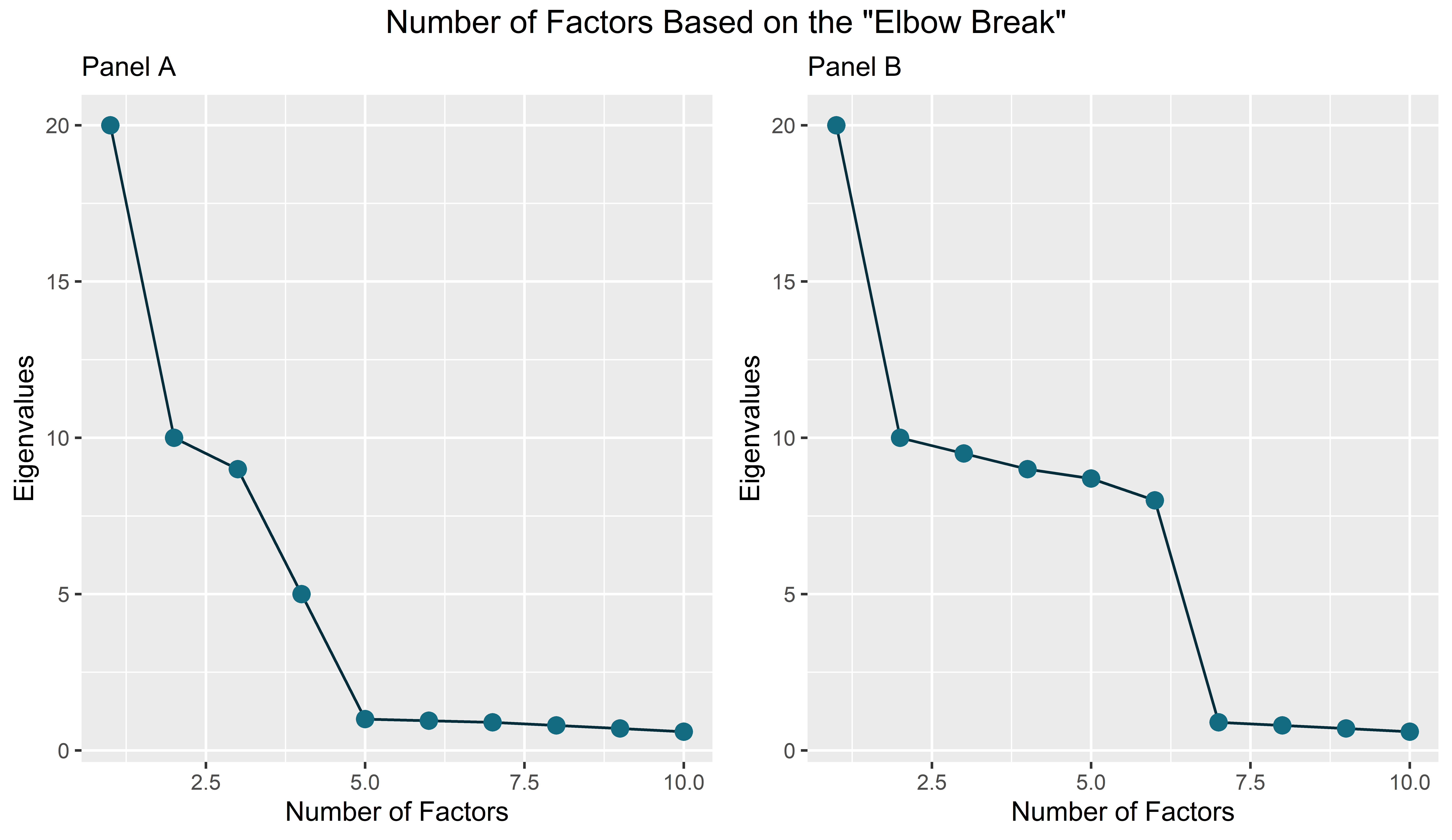
In Figure 7.1, one panel shows a relatively visible change in slope, whereas the other illustrates the main difficulty of the method: the elbow is not always obvious. Scree plots are therefore useful visual diagnostics, but factor retention should not rely on visual inspection alone.
7.3 Parallel Analysis
Parallel analysis, originally proposed by Horn (1965), compares the eigenvalues obtained from the observed data with eigenvalues obtained under a reference condition in which the variables do not share the factor structure present in the observed data.
The general logic is:
- obtain the factor eigenvalues from the observed data;
- repeatedly generate reference datasets in which the observed associations have been removed;
- obtain factor eigenvalues from each reference dataset; and
- retain factors whose observed eigenvalues are larger than the corresponding reference eigenvalues.
Rather than comparing the observed eigenvalues with the arbitrary value of 1, parallel analysis therefore asks whether a factor explains more common variation than would be expected from data without the observed factor structure (Horn, 1965).
For ordinal questionnaire items, the procedure can be conducted using polychoric rather than Pearson correlations. This keeps the factor- retention analysis consistent with the treatment of the items as ordered categorical variables.
An observed factor is more convincing when it explains more common variation than we would expect to obtain simply from random data.
Parallel analysis generally performs better than relying solely on the Kaiser rule or an informal scree decision (Zwick & Velicer, 1986).
7.4 Theory
Statistical retention rules are evidence, not substitutes for substantive reasoning. A retained factor should also make theoretical sense.
Suppose a theory proposes three distinguishable dimensions of behavioral intention, and the instrument was deliberately written to represent those three dimensions. A parallel analysis suggesting three factors would be especially informative because statistical and theoretical expectations converge. If the statistical procedures strongly disagree with the theoretical structure, the discrepancy itself becomes something to investigate.
A defensible factor-retention decision combines statistical evidence, factor interpretability, item content, and substantive theory. Parallel analysis is useful because it gives a stronger statistical reference point, but the final solution still needs substantive interpretation.
8 3. Factor Extraction
After deciding how many factors to retain, we estimate the common-factor solution. The extraction method determines how that solution is obtained from the observed correlations.
Common options include:
- maximum likelihood;
- principal-axis factoring;
- minimum residual methods;
- generalized least squares;
- unweighted least squares; and
- minimum-rank factor analysis.
When continuous variables are reasonably compatible with multivariate normality, maximum likelihood has useful statistical properties, including inferential tests and model-comparison possibilities (Fabrigar et al., 1999). When distributional assumptions are less plausible, other common-factor estimators may be more suitable.
For ordinal questionnaire items, the choice of correlation matrix is also important. Pearson correlations treat the observed categories as numerical values directly, whereas polychoric correlations attempt to represent the association between underlying continuous variables that generate ordered categorical responses. The estimator and the correlation matrix should therefore be selected together with the measurement characteristics of the items.
8.1 EFA Is Not PCA
Exploratory factor analysis is frequently confused with Principal Component Analysis (PCA), but they answer different questions (Fabrigar et al., 1999).
| Exploratory Factor Analysis | Principal Component Analysis |
|---|---|
| Models common variance among indicators | Decomposes total observed variance |
| Introduces latent common factors | Produces weighted composites of observed variables |
| Includes a unique component for each indicator | Does not separate common from unique variance in the common-factor sense |
| Appropriate when the goal is to model latent structure | Appropriate when the goal is primarily data reduction or composite construction |
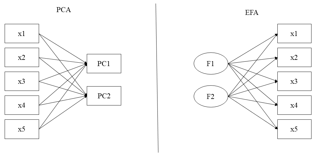
The distinction also connects with the discussion of latent-variable models in Chapter 3. EFA usually receives a reflective interpretation: variation in the common factor is used to account for covariation among its indicators. PCA does not require this latent common-cause interpretation.
Both procedures can produce loading-like matrices and low-dimensional summaries. Their mathematical goals are nevertheless different. If the research question concerns latent common factors, use a common-factor method rather than selecting PCA simply because it is available in the software.
9 4. Factor Rotation
After factors have been extracted, the initial solution is often difficult to interpret. Rotation searches for an equivalent representation in which the loading pattern is clearer.
The objective is usually a form of simple structure: ideally, an item has a relatively strong loading on the factor it represents and small loadings on the others.
There are two broad families of rotation:
| Rotation | Relationship among factors | Examples | When useful |
|---|---|---|---|
| Orthogonal | Factor correlations are fixed at zero | varimax, quartimax | When uncorrelated factors are substantively defensible |
| Oblique | Factors are allowed to correlate | oblimin, promax | Usually more realistic when psychological dimensions may be related |
Orthogonal rotation keeps the factor axes at 90°. Oblique rotation allows the axes to move away from 90°, permitting correlations among factors.
In psychological research, assuming that dimensions are exactly uncorrelated is often a strong assumption. When there is no compelling reason to impose orthogonality, an oblique rotation can be a useful starting point (Fabrigar et al., 1999).
With an oblique rotation, software may provide both a pattern matrix and a structure matrix. The pattern matrix contains the regression-like factor loadings, whereas the structure matrix contains correlations between variables and factors. When factors correlate, these matrices are not identical.
Rotation does not create a new substantive model out of nothing; it changes the orientation used to represent the retained factor space so that interpretation becomes easier. The rotated solution still has to be evaluated in relation to theory, item content, cross-loadings, and factor correlations.
10 Running an EFA in R
We will use the psych package (Revelle, 2023). The example uses the 25 personality items from the bfi dataset included in psych.
10.1 Install the Package
The installation only needs to be performed once.
Then load the packages:
10.2 Prepare the BFI Items
To make the rest of the tutorial easier to read, we first create one object containing the 25 BFI items and remove incomplete response patterns for this demonstration.
Complete-case deletion is used here to keep the tutorial simple. In a substantive analysis, the amount and mechanism of missingness should be examined rather than automatically deleting every participant with one missing item.
10.3 Data Adequacy in R
Because the BFI items are ordered response categories, we will use a polychoric correlation matrix consistently throughout the example.
10.3.1 Bartlett’s test
$chisq
[1] 23262.17

$p.value
[1] 0

$df
[1] 300
A small p-value indicates that the correlation matrix differs from an identity matrix. This provides evidence that there are nonzero associations available for a factor model to explain.
10.3.2 KMO
Kaiser-Meyer-Olkin factor adequacy
Call: psych::KMO(r = R_poly)
Overall MSA =  0.86
MSA for each item =
  A1   A2   A3   A4   A5   C1   C2   C3   C4   C5   E1   E2   E3   E4   E5   N1
0.77 0.84 0.88 0.88 0.91 0.86 0.80 0.86 0.84 0.87 0.84 0.89 0.90 0.88 0.90 0.78
  N2   N3   N4   N5   O1   O2   O3   O4   O5
0.78 0.87 0.89 0.86 0.88 0.80 0.86 0.78 0.79
The output reports both the overall KMO and the measure of sampling adequacy for each item. The latter is useful for identifying individual items that may not share much common information with the remainder of the item set.
10.4 Parallel Analysis in R
Because the BFI items are ordinal, we will conduct the parallel analysis using polychoric correlations. The psych::fa.parallel() function can calculate these correlations internally by specifying cor = "poly" (Revelle, 2023).
We also specify fa = "fa" because our objective is to determine the number of common factors, rather than the number of principal components.
Show parallel-analysis code
set.seed(2026)

parallel_results <- psych::fa.parallel(
  bfi_complete,
  fa = "fa",          # parallel analysis for factors, not components
  fm = "minres",      # minimum residual factor extraction
  cor = "poly",       # polychoric correlations
  n.iter = 50,       # number of random/resampled datasets, higher is better
  quant = .95,        # compare with the 95th percentile
  sim = TRUE,        # use randomized/resampled observed data
  plot = TRUE,
  main = "Parallel Analysis: BFI Items"
)
Parallel analysis suggests that the number of factors = 6 and the number of components = NA [1] 6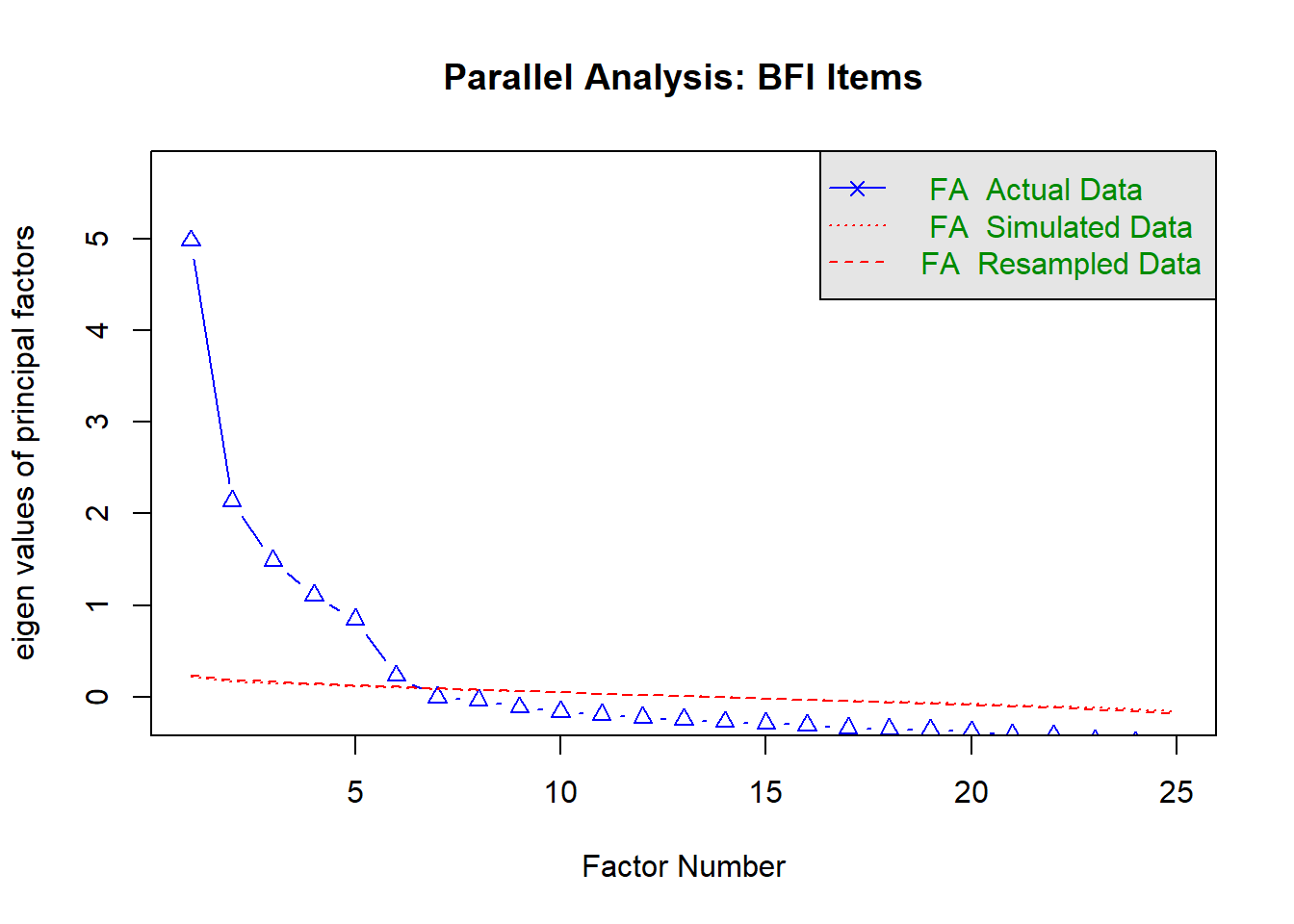
For the BFI, the expected substantive structure contains five broad personality dimensions. The parallel-analysis result can therefore be considered together with this theoretical expectation.
10.5 Extract the Factors
Suppose the retention evidence supports five factors. We can estimate a five-factor solution using minimum residual extraction and an oblique rotation:
Carregando namespace exigido: GPArotationHere:
-
nfactors = 5specifies the retained number of factors; -
n.obssupplies the number of participants; -
rotate = "oblimin"allows the factors to correlate; -
cor = "poly"uses polychoric correlations; and -
fm = "minres"uses minimum residual factor extraction.
The next step is not simply to look for a few large loadings. The solution should be interpreted as a whole: the loading pattern, cross-loadings, communalities, factor correlations, and model-adequacy statistics all provide different information about the factor structure (Fabrigar et al., 1999; Revelle, 2023).
10.6 Interpreting the Factor Analysis Output
The psych::fa() object contains substantially more information than the factor-loading matrix alone. A useful first display is:
Factor Analysis using method =  minres
Call: psych::fa(r = R_poly, nfactors = 5, n.obs = nrow(bfi_complete),
    rotate = "oblimin", fm = "minres", cor = "poly")
Standardized loadings (pattern matrix) based upon correlation matrix
   item   MR4   MR1   MR3   MR5   MR2   h2   u2 com
N1   16  0.87                         0.74 0.26 1.1
N2   17  0.81                         0.66 0.34 1.0
N3   18  0.74                         0.59 0.41 1.1
N5   20  0.52                         0.40 0.60 2.1
N4   19  0.50 -0.41                   0.55 0.45 2.3
E2   12       -0.70                   0.61 0.39 1.1
E4   14        0.63                   0.60 0.40 1.5
E1   11       -0.59                   0.39 0.61 1.2
E5   15        0.45                   0.46 0.54 2.7
E3   13        0.44              0.32 0.50 0.50 2.6
C2    7              0.70             0.51 0.49 1.2
C4    9             -0.69             0.55 0.45 1.1
C3    8              0.61             0.36 0.64 1.1
C5   10             -0.60             0.49 0.51 1.4
C1    6              0.59             0.40 0.60 1.2
A2    2                    0.70       0.54 0.46 1.0
A3    3                    0.70       0.61 0.39 1.1
A5    5                    0.56       0.53 0.47 1.5
A1    1                   -0.50       0.26 0.74 1.7
A4    4                    0.47       0.35 0.65 1.9
O3   23                          0.66 0.54 0.46 1.2
O5   25                         -0.59 0.36 0.64 1.2
O1   21                          0.57 0.39 0.61 1.1
O2   22                         -0.50 0.30 0.70 1.6
O4   24       -0.37              0.44 0.35 0.65 2.6

                       MR4  MR1  MR3  MR5  MR2
SS loadings           2.83 2.49 2.39 2.35 1.96
Proportion Var        0.11 0.10 0.10 0.09 0.08
Cumulative Var        0.11 0.21 0.31 0.40 0.48
Proportion Explained  0.24 0.21 0.20 0.20 0.16
Cumulative Proportion 0.24 0.44 0.64 0.84 1.00

 With factor correlations of
      MR4   MR1   MR3   MR5  MR2
MR4  1.00 -0.21 -0.19 -0.06 0.01
MR1 -0.21  1.00  0.25  0.32 0.15
MR3 -0.19  0.25  1.00  0.22 0.21
MR5 -0.06  0.32  0.22  1.00 0.20
MR2  0.01  0.15  0.21  0.20 1.00

Mean item complexity =  1.5
Test of the hypothesis that 5 factors are sufficient.

df null model =  300  with the objective function =  9.59 with Chi Square =  23262.17
df of  the model are 185  and the objective function was  0.92

The root mean square of the residuals (RMSR) is  0.02
The df corrected root mean square of the residuals is  0.03

The harmonic n.obs is  2436 with the empirical chi square  661.08  with prob <  9.7e-55
The total n.obs was  2436  with Likelihood Chi Square =  2225.9  with prob <  0

Tucker Lewis Index of factoring reliability =  0.856
RMSEA index =  0.067  and the 90 % confidence intervals are  0.065 0.07
BIC =  783.25
Fit based upon off diagonal values = 0.99
Measures of factor score adequacy
                                                   MR4  MR1  MR3  MR5  MR2
Correlation of (regression) scores with factors   0.93 0.85 0.86 0.85 0.85
Multiple R square of scores with factors          0.86 0.72 0.75 0.72 0.72
Minimum correlation of possible factor scores     0.73 0.43 0.49 0.44 0.44
sort = TRUE groups items according to the factor on which they have their largest loading, which makes the pattern easier to inspect. cut = .30 hides loadings smaller than .30 only in the printed output. Those smaller loadings are still estimated and remain part of the fitted solution.
Values such as .30, .40, or .50 are sometimes used as descriptive reference points for factor loadings, but there is no universal value that separates a “good” item from a “bad” one. Interpretation should consider loading magnitude, cross-loadings, item content, sample size, theory, and the purpose of the instrument.
10.6.1 Factor Loadings
A factor loading describes the estimated relation between an observed indicator and a factor under the common-factor model. Larger absolute loadings indicate a stronger relation between the item and that factor.
For example, imagine that part of the output looks like this:
This pattern would suggest that these items are strongly associated with the same factor.
A rough descriptive guide is:
| Absolute loading | Descriptive interpretation |
|---|---|
| around .20 | weak |
| around .30 | modest |
| around .40 | moderate |
| .50 or larger | relatively strong |
These values should be treated as descriptions rather than decision rules.
The sign also matters. A negative loading means that higher standing on the factor is associated with lower scores on that item. This can be expected for negatively worded or reverse-keyed items if they have not been recoded.
10.6.2 Primary Loadings
The largest absolute loading for an item is often called its primary loading.
For example:
Here, item1 has a clear primary association with MR1.
The factor label itself should come from the content of the items. MR1 does not inherently mean Agreeableness, Neuroticism, or any other construct. The substantive name is assigned after examining which items define the factor and how those items fit the theory.
10.6.3 Cross-Loadings
A cross-loading occurs when an item has meaningful loadings on more than one factor.
For example:
This item is related to both factors rather than clearly representing only one.
A cross-loading can indicate several things:
- the item contains content relevant to more than one construct;
- the factors overlap conceptually;
- the wording is ambiguous;
- the theoretical structure is more complex than expected; or
- the item genuinely reflects multiple psychological processes.
For this reason, a cross-loading is not automatically evidence that an item should be removed.
One useful descriptive check is the difference between the largest and second-largest absolute loadings. Compare:
with:
The first item has a much clearer factorial interpretation than the second.
Rules such as “remove every item with a cross-loading above .30” can produce an artificially simple scale while damaging content validity.
Instead ask:
- Is the secondary loading substantively meaningful?
- Is the primary loading clearly stronger than the secondary loading?
- Does the item intentionally represent overlapping content?
- Would removing the item narrow the construct being measured?
10.6.4 Communalities
psych::fa() reports the communality of each item in the h2 column.
The communality represents the proportion of an item’s standardized variance reproduced by the retained common factors.
For item (i),
\[ h_i^2 \]
denotes its communality.
In an orthogonal factor solution, the communality can be written as the sum of the squared loadings:
\[ h_i^2 = \lambda_{i1}^2 + \lambda_{i2}^2 + \cdots + \lambda_{im}^2. \]
With oblique factors, the factors are correlated, so the relationship also depends on the factor-correlation matrix.
Suppose an item has:
Approximately 64% of its standardized variance is represented by the common factor solution.
If another item has:
most of its variance is not represented by the retained common factors. This may indicate that the item is only weakly connected to the factor structure, although item content and theoretical importance should also be considered.
You can extract the communalities directly with:
       A1        A2        A3        A4        A5        C1        C2        C3
0.2601063 0.5407087 0.6055430 0.3546105 0.5306318 0.3973541 0.5055632 0.3601045
       C4        C5        E1        E2        E3        E4        E5        N1
0.5451009 0.4859517 0.3866555 0.6064446 0.4953139 0.6004587 0.4642264 0.7404081
       N2        N3        N4        N5        O1        O2        O3        O4
0.6587082 0.5925959 0.5490599 0.4023570 0.3915932 0.3010791 0.5396637 0.3499441
       O5
0.3604614
10.6.5 Uniqueness
The u2 column contains the uniqueness of each indicator.
For standardized indicators,
\[ u_i^2 = 1-h_i^2. \]
Thus, if
then
Approximately 36% of the item’s standardized variance remains outside the common factor solution.
This unique component contains both item-specific variance and measurement error.
In R:
       A1        A2        A3        A4        A5        C1        C2        C3
0.7398937 0.4592913 0.3944570 0.6453895 0.4693682 0.6026459 0.4944368 0.6398955
       C4        C5        E1        E2        E3        E4        E5        N1
0.4548991 0.5140483 0.6133445 0.3935554 0.5046861 0.3995413 0.5357736 0.2595919
       N2        N3        N4        N5        O1        O2        O3        O4
0.3412918 0.4074041 0.4509401 0.5976430 0.6084068 0.6989209 0.4603363 0.6500559
       O5
0.6395386
10.6.6 Factorial Complexity
The com column in the psych::fa() output summarizes factorial complexity.
Values close to 1 indicate that an item is mainly associated with one factor. Larger values indicate that its loading pattern is distributed across multiple factors.
For example:
suggests a relatively simple loading pattern, whereas
suggests that the item is meaningfully associated with more than one factor.
The complexity index is therefore a useful summary of the loading pattern, but it should not replace inspection of the individual loadings.
10.6.7 Factor Correlations
Because we used an oblique rotation,
the factors are allowed to correlate.
The factor-correlation matrix is stored in:
             MR4        MR1        MR3        MR5         MR2
MR4  1.000000000 -0.2126722 -0.1910156 -0.0575031 0.009609556
MR1 -0.212672198  1.0000000  0.2454965  0.3157042 0.145754015
MR3 -0.191015614  0.2454965  1.0000000  0.2155756 0.207027872
MR5 -0.057503100  0.3157042  0.2155756  1.0000000 0.203959770
MR2  0.009609556  0.1457540  0.2070279  0.2039598 1.000000000
For example:
A correlation of .42 indicates that the factors are related but still represent distinguishable dimensions.
Very high correlations can raise questions about whether two factors are empirically distinct. Correlations approaching .80 or .90, for example, may deserve closer inspection. This is not a universal threshold for combining factors: the theoretical distinction between the constructs also matters.
Psychological constructs are often related. Forcing their correlations to zero with an orthogonal rotation can distort the loading pattern. Oblique rotation allows those relationships to be represented directly.
10.6.8 Pattern Matrix and Structure Matrix
With oblique rotation, two loading-like matrices are relevant.
The pattern matrix contains the unique regression-like relation of each factor with each item while accounting for correlations among the factors. The loadings printed by psych::fa() are the pattern coefficients used for primary interpretation.
The structure matrix contains the correlations between the items and the factors.
When factors are correlated, these two matrices are not identical.
The structure matrix can be obtained from:
     MR4   MR1   MR3   MR5   MR2
A1  0.18  0.00 -0.04 -0.44 -0.11
A2 -0.08  0.26  0.24  0.73  0.18
A3 -0.10  0.37  0.23  0.76  0.21
A4 -0.13  0.29  0.32  0.52 -0.02
A5 -0.21  0.47  0.23  0.66  0.21
C1 -0.04  0.11  0.60  0.15  0.29
C2  0.05  0.09  0.68  0.20  0.21
C3 -0.07  0.09  0.59  0.19  0.06
C4  0.30 -0.20 -0.72 -0.14 -0.17
C5  0.33 -0.31 -0.64 -0.15 -0.04
E1  0.05 -0.60 -0.06 -0.28 -0.18
E2  0.26 -0.76 -0.25 -0.32 -0.19
E3 -0.01  0.55  0.22  0.45  0.44
E4 -0.16  0.72  0.22  0.49  0.09
E5  0.02  0.53  0.43  0.29  0.37
N1  0.85 -0.12 -0.17 -0.15 -0.05
N2  0.81 -0.16 -0.15 -0.12  0.02
N3  0.76 -0.24 -0.18  0.00  0.01
N4  0.61 -0.50 -0.29 -0.07  0.03
N5  0.55 -0.29 -0.16  0.09 -0.16
O1 -0.03  0.21  0.23  0.18  0.61
O2  0.19 -0.04 -0.19  0.04 -0.48
O3 -0.01  0.30  0.20  0.27  0.70
O4  0.21 -0.28 -0.02  0.16  0.42
O5  0.10 -0.01 -0.16 -0.06 -0.58
An item may therefore have a modest pattern loading on a factor but a larger structure coefficient because that factor correlates with another factor associated with the item.
For an oblique solution, the pattern matrix is usually the main matrix used to interpret which factor is uniquely associated with each item.
10.6.9 Variance Explained by the Factors
The printed output also includes a section similar to:
These quantities help describe the relative contribution of the retained factors.
SS loadings summarize the amount of variance associated with the loadings for each factor.
Proportion Var expresses that amount relative to the total standardized variance of the indicators.
Proportion Explained expresses each factor’s contribution relative to the variance explained by the retained factors.
These statistics are useful descriptions of the solution, but a factor should not be judged as psychologically important only because it accounts for more variance than another factor.
10.7 Model Adequacy
An interpretable loading matrix is not enough. We should also ask how well the factor solution reproduces the observed correlation matrix.
Let
\[ R \]
represent the observed polychoric correlation matrix and
\[ \hat{R} \]
the correlations reproduced by the fitted factor model. The residual correlation matrix is
\[ R-\hat{R}. \]
psych::fa() reports several statistics related to this reproduction.
10.7.1 Residual Correlations and RMSR
The Root Mean Square Residual (RMSR) summarizes the average size of the residual correlations.
Smaller RMSR values indicate that the retained factor solution reproduces the observed correlations more closely.
The residuals can be inspected directly:
   A1    A2    A3    A4    A5    C1    C2    C3    C4    C5    E1
A1  0.74
A2 -0.10  0.46
A3 -0.01  0.01  0.39
A4  0.02  0.01  0.02  0.65
A5  0.04 -0.04  0.03 -0.01  0.47
C1  0.02 -0.03 -0.01 -0.05  0.04  0.60
C2  0.04 -0.04 -0.02  0.05  0.00  0.06  0.49
C3  0.03  0.04 -0.01 -0.05  0.01  0.01 -0.01  0.64
C4  0.09 -0.02  0.00  0.01  0.02  0.00  0.01  0.01  0.45
C5  0.01  0.01 -0.01 -0.04  0.01  0.05  0.05 -0.02  0.05  0.51
E1  0.07 -0.04  0.04  0.02  0.05  0.00  0.03  0.01  0.07 -0.04  0.61
E2  0.04 -0.02  0.01  0.02  0.03  0.01  0.01  0.00  0.03  0.01  0.06
E3  0.07 -0.05  0.03  0.00  0.05 -0.02  0.02  0.01  0.04 -0.02  0.04
E4  0.05 -0.05 -0.03  0.02  0.05  0.06  0.03 -0.01  0.03  0.02 -0.03
E5  0.00  0.07 -0.01 -0.02 -0.02  0.01  0.00  0.02  0.01  0.01 -0.01
N1 -0.03  0.02  0.03  0.02 -0.02 -0.04 -0.04 -0.01 -0.02 -0.04  0.00
N2 -0.03  0.05  0.03 -0.02 -0.02 -0.02 -0.03 -0.01 -0.05  0.01 -0.02
N3  0.00 -0.02 -0.01  0.02  0.00  0.01 -0.02 -0.02 -0.02 -0.02 -0.01
N4  0.01 -0.02 -0.01 -0.02  0.01  0.00  0.03  0.00  0.00  0.02  0.03
N5 -0.01 -0.01 -0.05  0.00  0.01  0.01  0.05  0.00  0.02 -0.01 -0.07
O1  0.06  0.00  0.00  0.02  0.00 -0.01  0.02  0.02  0.06  0.00  0.05
O2  0.05  0.00 -0.02 -0.02  0.02  0.02  0.04  0.03  0.06  0.05  0.03
O3  0.01 -0.03  0.00  0.01  0.01  0.00  0.05  0.00  0.05  0.00  0.00
O4  0.00  0.00 -0.03 -0.01  0.00  0.04 -0.01  0.03  0.03  0.02  0.01
O5  0.05 -0.04  0.01  0.00  0.01  0.02  0.03  0.04  0.07  0.01  0.05
   E2    E3    E4    E5    N1    N2    N3    N4    N5    O1    O2
E2  0.39
E3  0.02  0.50
E4 -0.02  0.01  0.40
E5  0.00  0.01 -0.05  0.54
N1  0.01 -0.02 -0.04  0.02  0.26
N2  0.02 -0.04 -0.02  0.03  0.08  0.34
N3 -0.04  0.01  0.01 -0.04 -0.01 -0.01  0.41
N4 -0.04  0.02  0.01 -0.02 -0.03 -0.05  0.06  0.45
N5  0.02  0.01  0.02 -0.05 -0.02 -0.04  0.03  0.03  0.60
O1  0.03  0.05  0.01  0.04 -0.01 -0.03 -0.02  0.01 -0.02  0.61
O2  0.02  0.04  0.03  0.03 -0.03  0.00 -0.04 -0.01  0.01  0.01  0.70
O3  0.01  0.03  0.02 -0.02  0.00 -0.02 -0.02 -0.01  0.04  0.00 -0.03
O4  0.02  0.01  0.04  0.00 -0.02  0.00 -0.01 -0.01  0.01  0.04  0.05
O5  0.03  0.04  0.04  0.02 -0.01 -0.05 -0.02  0.01  0.01  0.03  0.06
   O3    O4    O5
O3  0.46
O4  0.00  0.65
O5  0.01  0.00  0.64
This is useful because a single global statistic can hide localized misfit. Large residual correlations identify particular item pairs whose association is not reproduced well by the factor model.
The RMSR itself is available as:
10.7.2 RMSEA
psych::fa() also reports the Root Mean Square Error of Approximation (RMSEA).
RMSEA incorporates model discrepancy and degrees of freedom. Smaller values indicate less approximate misfit.
The output usually includes both the estimate and a confidence interval. The interval is important because RMSEA is an estimated quantity rather than a perfectly known property of the population.
You can inspect it directly with:
Values such as .05, .06, or .08 are often used as descriptive benchmarks, but they should not be treated as universal decision thresholds. Their behavior depends on features such as sample size, number of variables, factor structure, and estimator.
10.7.3 Tucker–Lewis Index
The Tucker–Lewis Index (TLI) compares the fitted factor solution with a more restrictive baseline model while also accounting for model complexity.
Values closer to 1 indicate greater improvement relative to the baseline model.
In R:
Values such as .90 or .95 are often used as descriptive reference points, but the same caution applies: they should not function as automatic pass/fail rules.
10.7.4 Chi-Square Test
The chi-square statistic evaluates whether the model reproduces the population correlation structure exactly.
A statistically significant chi-square provides evidence against exact fit. With large samples, however, even relatively small discrepancies can become statistically significant.
For this reason, the chi-square test is best interpreted together with the residuals, approximate-fit indices, loading pattern, and substantive interpretation.
10.7.5 Bayesian Information Criterion
psych::fa() also reports the Bayesian Information Criterion (BIC).
BIC is most useful for comparing alternative factor solutions fitted to the same data. Smaller values indicate a better balance between fit and model complexity.
The absolute BIC value is not especially informative by itself. For example, we could compare four- and five-factor solutions:
BIC_4_factors BIC_5_factors
    2774.4605      783.2508
A smaller BIC for one solution provides one piece of evidence favoring that solution, but factor retention should still incorporate the parallel analysis, loading pattern, and theoretical interpretability.
10.7.6 Reproduced Correlations
The observed polychoric correlations were stored earlier as:
             A1            A2          A3          A4          A5          C1
A1  1.000000000 -0.4211375789 -0.33259604 -0.18668402 -0.24123660 -0.01377998
A2 -0.421137579  1.0000000000  0.57304664  0.40736058  0.45586315  0.12539211
A3 -0.332596035  0.5730466423  1.00000000  0.43450257  0.58196486  0.14335733
A4 -0.186684018  0.4073605839  0.43450257  1.00000000  0.37318208  0.11683742
A5 -0.241236598  0.4558631454  0.58196486  0.37318208  1.00000000  0.17447818
C1 -0.013779980  0.1253921078  0.14335733  0.11683742  0.17447818  1.00000000
C2  0.005088399  0.1517415313  0.16326874  0.26298855  0.14320042  0.49235344
C3 -0.023638034  0.2215743513  0.15749332  0.16749272  0.15344229  0.35276862
C4  0.138258272 -0.1895623205 -0.16407935 -0.21529382 -0.16626419 -0.42271819
C5  0.047037168 -0.1541521299 -0.18807167 -0.29241180 -0.19869661 -0.30283583
E1  0.118616152 -0.2553540684 -0.24678157 -0.15893091 -0.27948642 -0.03645343
E2  0.104140375 -0.2841864510 -0.33798921 -0.23522606 -0.38645837 -0.12338872
E3 -0.068069817  0.2963505373  0.44506770  0.23576037  0.47346481  0.16146069
E4 -0.085044803  0.3286985129  0.42767864  0.36660727  0.53509346  0.16432293
E5 -0.025038503  0.3210939732  0.29538214  0.19715503  0.29920487  0.29994887
N1  0.188509751 -0.1205353306 -0.10941261 -0.12529805 -0.23652158 -0.08973131
N2  0.161422715 -0.0663232717 -0.10173960 -0.16572104 -0.22457880 -0.04372437
N3  0.103818764 -0.0539845636 -0.06131410 -0.07947288 -0.16025242 -0.03424998
N4  0.049690417 -0.1122390114 -0.14363846 -0.19531364 -0.23140285 -0.10751997
N5  0.008526750  0.0206904708 -0.05253098 -0.01396088 -0.09422165 -0.06281609
O1 -0.011649997  0.1561393896  0.18822211  0.06737125  0.19934755  0.22240906
O2  0.068671156  0.0007047078 -0.02134599  0.03684173 -0.02057077 -0.15657428
O3 -0.091220761  0.1917570367  0.26768225  0.08115293  0.27377762  0.22716088
O4 -0.111654046  0.1078295788  0.05642647 -0.05892290  0.01808457  0.12701050
O5  0.118628553 -0.1020166147 -0.06687794  0.03516019 -0.06673795 -0.17385214
             C2           C3          C4          C5           E1          E2
A1  0.005088399 -0.023638034  0.13825827  0.04703717  0.118616152  0.10414038
A2  0.151741531  0.221574351 -0.18956232 -0.15415213 -0.255354068 -0.28418645
A3  0.163268736  0.157493317 -0.16407935 -0.18807167 -0.246781568 -0.33798921
A4  0.262988552  0.167492722 -0.21529382 -0.29241180 -0.158930912 -0.23522606
A5  0.143200420  0.153442287 -0.16626419 -0.19869661 -0.279486420 -0.38645837
C1  0.492353445  0.352768623 -0.42271819 -0.30283583 -0.036453430 -0.12338872
C2  1.000000000  0.401773012 -0.44931225 -0.33681783  0.011661807 -0.09056640
C3  0.401773012  1.000000000 -0.40129491 -0.39252413 -0.003263281 -0.09872245
C4 -0.449312248 -0.401294909  1.00000000  0.54002343  0.114233569  0.24261444
C5 -0.336817831 -0.392524127  0.54002343  1.00000000  0.074569753  0.29797016
E1  0.011661807 -0.003263281  0.11423357  0.07456975  1.000000000  0.51577923
E2 -0.090566396 -0.098722451  0.24261444  0.29797016  0.515779226  1.00000000
E3  0.185314132  0.109803501 -0.10914629 -0.18220838 -0.348552968 -0.42886590
E4  0.141156529  0.111954302 -0.13921733 -0.23449388 -0.481025772 -0.58575414
E5  0.305614234  0.237799844 -0.27947011 -0.27183105 -0.339813901 -0.43076604
N1 -0.020443333 -0.086311782  0.24334296  0.23648877  0.019119553  0.19432680
N2  0.005682253 -0.071535407  0.17927363  0.27237407  0.018878821  0.22113712
N3  0.004642540 -0.087414133  0.22948378  0.26417435  0.057463626  0.20901330
N4 -0.039702682 -0.127351533  0.30043503  0.38517183  0.256697231  0.38632321
N5  0.049910916 -0.029398457  0.22808217  0.20913228  0.059788079  0.28793433
O1  0.200037093  0.112002817 -0.11830016 -0.10335774 -0.125149301 -0.18704329
O2 -0.078857766 -0.037283834  0.23827570  0.14985494  0.060972909  0.09894203
O3  0.225559988  0.066498848 -0.10959210 -0.09285602 -0.239067093 -0.26912186
O4  0.067278775  0.025082028  0.06414477  0.16108227  0.107078442  0.20314059
O5 -0.107280679 -0.015591700  0.22079775  0.06674445  0.090917046  0.09302565
            E3          E4           E5          N1           N2          N3
A1 -0.06806982 -0.08504480 -0.025038503  0.18850975  0.161422715  0.10381876
A2  0.29635054  0.32869851  0.321093973 -0.12053533 -0.066323272 -0.05398456
A3  0.44506770  0.42767864  0.295382143 -0.10941261 -0.101739605 -0.06131410
A4  0.23576037  0.36660727  0.197155032 -0.12529805 -0.165721038 -0.07947288
A5  0.47346481  0.53509346  0.299204874 -0.23652158 -0.224578804 -0.16025242
C1  0.16146069  0.16432293  0.299948867 -0.08973131 -0.043724373 -0.03424998
C2  0.18531413  0.14115653  0.305614234 -0.02044333  0.005682253  0.00464254
C3  0.10980350  0.11195430  0.237799844 -0.08631178 -0.071535407 -0.08741413
C4 -0.10914629 -0.13921733 -0.279470107  0.24334296  0.179273629  0.22948378
C5 -0.18220838 -0.23449388 -0.271831055  0.23648877  0.272374066  0.26417435
E1 -0.34855297 -0.48102577 -0.339813901  0.01911955  0.018878821  0.05746363
E2 -0.42886590 -0.58575414 -0.430766038  0.19432680  0.221137122  0.20901330
E3  1.00000000  0.46148611  0.439962621 -0.05365127 -0.060101416 -0.01680078
E4  0.46148611  1.00000000  0.354744716 -0.15976895 -0.168629793 -0.14542409
E5  0.43996262  0.35474472  1.000000000  0.04263309  0.051704557 -0.06554064
N1 -0.05365127 -0.15976895  0.042633089  1.00000000  0.775301157  0.62091329
N2 -0.06010142 -0.16862979  0.051704557  0.77530116  1.000000000  0.59917701
N3 -0.01680078 -0.14542409 -0.065540640  0.62091329  0.599177012  1.00000000
N4 -0.15651793 -0.34044139 -0.219074530  0.44989682  0.431173086  0.56781191
N5 -0.09914653 -0.13006463 -0.164021538  0.42111846  0.385328612  0.47445915
O1  0.38187454  0.16858405  0.342670623 -0.06441975 -0.044226047 -0.04974806
O2 -0.10026908  0.04504703 -0.112343752  0.14692170  0.129122710  0.11182084
O3  0.45386977  0.24095100  0.346380056 -0.04900868 -0.026995254 -0.03253343
O4  0.08243746 -0.11658531  0.006142618  0.09273774  0.155926480  0.19278776
O5 -0.15738083  0.04963259 -0.146785157  0.11758313  0.020909256  0.05477021
            N4          N5          O1            O2          O3           O4
A1  0.04969042  0.00852675 -0.01165000  0.0686711561 -0.09122076 -0.111654046
A2 -0.11223901  0.02069047  0.15613939  0.0007047078  0.19175704  0.107829579
A3 -0.14363846 -0.05253098  0.18822211 -0.0213459932  0.26768225  0.056426468
A4 -0.19531364 -0.01396088  0.06737125  0.0368417307  0.08115293 -0.058922904
A5 -0.23140285 -0.09422165  0.19934755 -0.0205707654  0.27377762  0.018084566
C1 -0.10751997 -0.06281609  0.22240906 -0.1565742799  0.22716088  0.127010500
C2 -0.03970268  0.04991092  0.20003709 -0.0788577657  0.22555999  0.067278775
C3 -0.12735153 -0.02939846  0.11200282 -0.0372838338  0.06649885  0.025082028
C4  0.30043503  0.22808217 -0.11830016  0.2382756999 -0.10959210  0.064144768
C5  0.38517183  0.20913228 -0.10335774  0.1498549408 -0.09285602  0.161082273
E1  0.25669723  0.05978808 -0.12514930  0.0609729089 -0.23906709  0.107078442
E2  0.38632321  0.28793433 -0.18704329  0.0989420298 -0.26912186  0.203140590
E3 -0.15651793 -0.09914653  0.38187454 -0.1002690834  0.45386977  0.082437459
E4 -0.34044139 -0.13006463  0.16858405  0.0450470259  0.24095100 -0.116585313
E5 -0.21907453 -0.16402154  0.34267062 -0.1123437515  0.34638006  0.006142618
N1  0.44989682  0.42111846 -0.06441975  0.1469217009 -0.04900868  0.092737737
N2  0.43117309  0.38532861 -0.04422605  0.1291227101 -0.02699525  0.155926480
N3  0.56781191  0.47445915 -0.04974806  0.1118208391 -0.03253343  0.192787757
N4  1.00000000  0.44644119 -0.04706704  0.0794304952 -0.06679344  0.268377160
N5  0.44644119  1.00000000 -0.15483690  0.2132289765 -0.10447257  0.137311942
O1 -0.04706704 -0.15483690  1.00000000 -0.2820873778  0.45280036  0.248944460
O2  0.07943050  0.21322898 -0.28208738  1.0000000000 -0.34252993 -0.106602854
O3 -0.06679344 -0.10447257  0.45280036 -0.3425299285  1.00000000  0.247832115
O4  0.26837716  0.13731194  0.24894446 -0.1066028544  0.24783211  1.000000000
O5  0.03096881  0.16029532 -0.31036937  0.3734435364 -0.37320281 -0.249788261
            O5
A1  0.11862855
A2 -0.10201661
A3 -0.06687794
A4  0.03516019
A5 -0.06673795
C1 -0.17385214
C2 -0.10728068
C3 -0.01559170
C4  0.22079775
C5  0.06674445
E1  0.09091705
E2  0.09302565
E3 -0.15738083
E4  0.04963259
E5 -0.14678516
N1  0.11758313
N2  0.02090926
N3  0.05477021
N4  0.03096881
N5  0.16029532
O1 -0.31036937
O2  0.37344354
O3 -0.37320281
O4 -0.24978826
O5  1.00000000
The fitted factor model attempts to reproduce those relationships. Residuals show where the reproduction is weaker:
   A1    A2    A3    A4    A5    C1    C2    C3    C4    C5    E1
A1  0.74
A2 -0.10  0.46
A3 -0.01  0.01  0.39
A4  0.02  0.01  0.02  0.65
A5  0.04 -0.04  0.03 -0.01  0.47
C1  0.02 -0.03 -0.01 -0.05  0.04  0.60
C2  0.04 -0.04 -0.02  0.05  0.00  0.06  0.49
C3  0.03  0.04 -0.01 -0.05  0.01  0.01 -0.01  0.64
C4  0.09 -0.02  0.00  0.01  0.02  0.00  0.01  0.01  0.45
C5  0.01  0.01 -0.01 -0.04  0.01  0.05  0.05 -0.02  0.05  0.51
E1  0.07 -0.04  0.04  0.02  0.05  0.00  0.03  0.01  0.07 -0.04  0.61
E2  0.04 -0.02  0.01  0.02  0.03  0.01  0.01  0.00  0.03  0.01  0.06
E3  0.07 -0.05  0.03  0.00  0.05 -0.02  0.02  0.01  0.04 -0.02  0.04
E4  0.05 -0.05 -0.03  0.02  0.05  0.06  0.03 -0.01  0.03  0.02 -0.03
E5  0.00  0.07 -0.01 -0.02 -0.02  0.01  0.00  0.02  0.01  0.01 -0.01
N1 -0.03  0.02  0.03  0.02 -0.02 -0.04 -0.04 -0.01 -0.02 -0.04  0.00
N2 -0.03  0.05  0.03 -0.02 -0.02 -0.02 -0.03 -0.01 -0.05  0.01 -0.02
N3  0.00 -0.02 -0.01  0.02  0.00  0.01 -0.02 -0.02 -0.02 -0.02 -0.01
N4  0.01 -0.02 -0.01 -0.02  0.01  0.00  0.03  0.00  0.00  0.02  0.03
N5 -0.01 -0.01 -0.05  0.00  0.01  0.01  0.05  0.00  0.02 -0.01 -0.07
O1  0.06  0.00  0.00  0.02  0.00 -0.01  0.02  0.02  0.06  0.00  0.05
O2  0.05  0.00 -0.02 -0.02  0.02  0.02  0.04  0.03  0.06  0.05  0.03
O3  0.01 -0.03  0.00  0.01  0.01  0.00  0.05  0.00  0.05  0.00  0.00
O4  0.00  0.00 -0.03 -0.01  0.00  0.04 -0.01  0.03  0.03  0.02  0.01
O5  0.05 -0.04  0.01  0.00  0.01  0.02  0.03  0.04  0.07  0.01  0.05
   E2    E3    E4    E5    N1    N2    N3    N4    N5    O1    O2
E2  0.39
E3  0.02  0.50
E4 -0.02  0.01  0.40
E5  0.00  0.01 -0.05  0.54
N1  0.01 -0.02 -0.04  0.02  0.26
N2  0.02 -0.04 -0.02  0.03  0.08  0.34
N3 -0.04  0.01  0.01 -0.04 -0.01 -0.01  0.41
N4 -0.04  0.02  0.01 -0.02 -0.03 -0.05  0.06  0.45
N5  0.02  0.01  0.02 -0.05 -0.02 -0.04  0.03  0.03  0.60
O1  0.03  0.05  0.01  0.04 -0.01 -0.03 -0.02  0.01 -0.02  0.61
O2  0.02  0.04  0.03  0.03 -0.03  0.00 -0.04 -0.01  0.01  0.01  0.70
O3  0.01  0.03  0.02 -0.02  0.00 -0.02 -0.02 -0.01  0.04  0.00 -0.03
O4  0.02  0.01  0.04  0.00 -0.02  0.00 -0.01 -0.01  0.01  0.04  0.05
O5  0.03  0.04  0.04  0.02 -0.01 -0.05 -0.02  0.01  0.01  0.03  0.06
   O3    O4    O5
O3  0.46
O4  0.00  0.65
O5  0.01  0.00  0.64
A solution can have visually appealing factor loadings while still reproducing some correlations poorly. This is why EFA interpretation should include both the factor pattern and model adequacy.
10.8 A Practical Order for Interpreting the Solution
A useful sequence is:
Inspect the loading pattern.
Which items define each factor?Identify cross-loadings.
Do some items have meaningful associations with multiple factors?Inspect communalities and uniquenesses.
How much of each item’s variance is represented by the retained factors?Inspect factorial complexity.
Are the items primarily associated with one factor, or is the loading pattern diffuse?Inspect factor correlations.
Are the factors related but still substantively distinguishable?Examine residuals and global model adequacy.
How well does the retained factor solution reproduce the observed polychoric correlations?Return to item content and theory.
Can the factors be given coherent psychological interpretations?
This final step is essential. A statistical procedure can identify five factors, but the numbers alone cannot tell us that those factors necessarily correspond to the five psychological constructs proposed by the researcher. The meaning of a factor comes from the indicators and the theory used to interpret their common variation.
A strong EFA solution is not defined by every loading exceeding .40, every communality exceeding .50, RMSEA falling below one cutoff, or the parallel analysis reproducing the theoretically expected number of factors exactly.
Instead, look for convergence among factor-retention evidence, coherent primary loadings, interpretable cross-loadings, reasonable communalities, distinguishable factor correlations, adequate reproduction of the correlation matrix, and a structure that makes substantive sense.
11 A Compact EFA Decision Guide
| Decision | Prefer asking… | Avoid… |
|---|---|---|
| Data adequacy | Are the items sufficiently related and theoretically suitable for common-factor modeling? | Treating Bartlett p < .05 as automatic permission to factor |
| Number of factors | Do parallel analysis, theory, and interpretability converge? | Using eigenvalue > 1 alone |
| Extraction | Which estimator fits the item type and distributional assumptions? | Using PCA when the research question concerns latent factors |
| Rotation | Is it reasonable to assume the psychological dimensions are exactly uncorrelated? | Choosing varimax automatically |
| Interpretation | Does the complete loading pattern make substantive sense? | Deleting items mechanically from a single loading cutoff |
| Reporting | Can readers reconstruct the major analytic decisions? | Reporting only the final number of factors |
12 How to Report an Exploratory Factor Analysis
A useful EFA report should make the analytic decisions transparent rather than merely state that “an EFA was conducted.”
At minimum, report:
- the variables/items included;
- the analytic sample size;
- the correlation matrix used (e.g., Pearson or polychoric);
- Bartlett’s test and KMO, if used;
- the factor-retention procedure;
- the extraction method;
- the rotation method;
- the retained number of factors;
- the relevant factor loadings and cross-loadings;
- factor correlations when using an oblique rotation; and
- any model-adequacy statistics used in interpretation.
For the BFI tutorial, the prose could follow this structure:
An exploratory factor analysis was conducted on the 25 BFI items using polychoric correlations and minimum residual factor analysis. The suitability of the correlation matrix was examined using Bartlett’s test of sphericity and the Kaiser–Meyer–Olkin measure. The number of factors was evaluated using parallel analysis with 500 simulated datasets and the 95th-percentile criterion. A five-factor solution was then extracted and rotated using oblimin, allowing correlations among factors. Factor loadings, cross-loadings, factor correlations, and model-adequacy statistics were considered jointly when interpreting the solution.
Insert the actual statistics from your analysis rather than relying on a generic cutoff or copying values from another study.
EFA provides evidence concerning internal structure. A five-factor solution that resembles the expected theory is useful evidence, but it does not establish content validity, response-process validity, relations with external variables, or the appropriateness of every proposed use of the scores.
13 Concluding Remarks
EFA is often introduced as a sequence of software commands, but the most important decisions happen before and after the extraction itself. The researcher must decide whether a common-factor model is substantively appropriate, how many factors to retain, which correlation and extraction methods fit the data, whether factors should be allowed to correlate, and whether the final solution is interpretable in light of the theory.
The key idea is therefore not simply to “find the number of factors.” EFA is a model-based way of asking whether a set of observed indicators can be represented by a smaller latent structure. Statistical procedures such as KMO, parallel analysis, extraction, and rotation help answer parts of that question, but no single statistic determines the psychological meaning of the factors.
The next chapter turns from this exploratory setting to confirmatory factor analysis, where the measurement structure is specified more explicitly and evaluated as a hypothesized model.