8 Social Desirability Bias
Self-report measures are central to research in psychology, education, health, and the social sciences. They are efficient and often provide access to behaviors, evaluations, feelings, and experiences that are not directly observable (Lange & Dewitte, 2019; Peterson & Kerin, 1981). At the same time, responses to self-report items can reflect more than the construct the researcher intends to measure.
Among these additional influences are response styles and response biases. Social desirability, acquiescence, and extreme responding are common examples. These influences matter because they can change item means, associations among items, factor structures, and relations with external variables.
This chapter distinguishes faking from socially desirable responding, examines how social desirability can enter a psychometric model, and reviews several strategies for controlling it:
- social-desirability scales;
- factor-analytic response-bias models;
- factor-mixture models;
- common-method-factor models; and
- Peabody-style balanced quadruplets and MIMIC modeling.
The final section implements two of these approaches in R.
8.1 Faking: Context, Motivation, and Opportunity
Faking is best understood as a context-dependent response behavior. A respondent deliberately changes answers in order to produce a self-presentation that serves some objective (Ziegler et al., 2011). The behavior is therefore not determined only by the person or only by the questionnaire. It emerges from an interaction among individual characteristics, situational demands, and features of the assessment itself.
Two broad forms are often distinguished:
| Form | General purpose |
|---|---|
| Faking good | Presenting oneself more favorably than one would under ordinary responding |
| Faking bad | Fabricating or exaggerating undesirable characteristics or symptoms for a desired outcome |
Faking good has been studied extensively in personality and selection contexts (Zickar & Robie, 1999). Faking bad is especially relevant when the respondent may benefit from appearing more impaired or symptomatic (Ziegler et al., 2011).
8.1.1 Why would a person fake?
The expectancy-based account summarized by Ziegler et al. (2011) emphasizes three kinds of beliefs:
- Can I do it? — the respondent believes that changing the intended impression is possible;
- Will it matter? — the respondent believes that altered responses can affect the outcome; and
- Do I value that outcome? — the resulting benefit is sufficiently important.
These beliefs can be influenced by personality, cognitive ability, knowledge of the construct being assessed, item transparency, previous testing experience, and characteristics of the testing situation (McFarland & Ryan, 2000; Raymark & Tafero, 2009; Riggio et al., 1988; Snell et al., 1999).
Faking refers to an intentional response process in a particular context. Social desirability is broader: it concerns the tendency for responses to be related to the social evaluation of the content. A high score on a social-desirability scale should therefore not automatically be interpreted as proof that a respondent lied.
8.6 Peabody Quadruplets: Separating Descriptive and Evaluative Content
A different strategy addresses social desirability during item construction. Peabody (1967) distinguished the descriptive content of a trait term from its evaluative desirability. By crossing low versus high descriptive content with low versus high evaluative content, researchers can construct balanced quadruplets.
| Low desirability | High desirability | |
|---|---|---|
| Low descriptive pole | Withdrawn | Introspective |
| High descriptive pole | Chatty | Communicative |
The design can also help separate acquiescence because positive and negative descriptive poles are represented within the same balanced set (Mirowsky & Ross, 1991).
For a four-item quadruplet, a simplified two-factor representation is
\[ \begin{bmatrix} x_1\\ x_2\\ x_3\\ x_4 \end{bmatrix} = \begin{bmatrix} -\lambda_{1c} & +\lambda_{1d}\\ -\lambda_{2c} & -\lambda_{2d}\\ +\lambda_{3c} & +\lambda_{3d}\\ +\lambda_{4c} & -\lambda_{4d} \end{bmatrix} \begin{bmatrix} \eta_c\\ \eta_d \end{bmatrix} + \begin{bmatrix} \epsilon_1\\ \epsilon_2\\ \epsilon_3\\ \epsilon_4 \end{bmatrix}, \]
where \(\eta_c\) represents descriptive content and \(\eta_d\) represents evaluative desirability. Related adjective-based approaches have used this logic to distinguish evaluative and descriptive personality variance (Pettersson et al., 2012, 2014; Saucier et al., 2001).
8.6.1 Extending the desirability factor with a MIMIC model
Degobi & Valentini (2023) evaluated whether a desirability factor identified from manipulated quadruplets could predict desirability effects in additional items through a Multiple Indicators Multiple Causes (MIMIC) model. Their simulation studies considered Likert-type and forced-choice versions of the approach and evaluated recovery using bias and coverage criteria.
The practical idea is:
- identify the desirability factor using items in which evaluative content was deliberately manipulated;
- estimate the substantive content factors from all relevant items; and
- regress additional, non-quadruplet items on the desirability factor.
This avoids requiring every item in a scale to be written as a quadruplet, although the method still depends on the quality and number of the manipulated quadruplets.
Two simulation tools were developed for planning these models: quadSimple, intended for early-stage design when little parameter information is available, and quadSim, intended for settings in which researchers already have more detailed information about the expected model parameters.
9 Controlling Social Desirability in R
9.1 Ferrando et al.’s Procedure with vampyr
The vampyr package implements factor-analytic procedures for controlling response bias (Navarro-Gonzalez et al., 2021).
Installation is required only once:
Load the package and inspect its example dataset:
       V2              V8             V13             V21
 Min.   :1.000   Min.   :1.000   Min.   :1.000   Min.   :1.000
 1st Qu.:3.000   1st Qu.:2.000   1st Qu.:1.000   1st Qu.:2.000
 Median :4.000   Median :4.000   Median :2.000   Median :3.000
 Mean   :3.667   Mean   :3.263   Mean   :2.317   Mean   :2.947
 3rd Qu.:5.000   3rd Qu.:4.000   3rd Qu.:3.000   3rd Qu.:4.000
 Max.   :5.000   Max.   :5.000   Max.   :5.000   Max.   :5.000
       V1              V6             V17            V19             V20
 Min.   :1.000   Min.   :1.000   Min.   :1.00   Min.   :1.000   Min.   :1.000
 1st Qu.:3.000   1st Qu.:1.000   1st Qu.:3.00   1st Qu.:3.000   1st Qu.:1.000
 Median :4.000   Median :2.000   Median :4.00   Median :4.000   Median :2.000
 Mean   :3.643   Mean   :2.467   Mean   :3.71   Mean   :3.493   Mean   :1.997
 3rd Qu.:5.000   3rd Qu.:3.000   3rd Qu.:5.00   3rd Qu.:5.000   3rd Qu.:3.000
 Max.   :5.000   Max.   :5.000   Max.   :5.00   Max.   :5.000   Max.   :5.000
      V25
 Min.   :1.000
 1st Qu.:1.000
 Median :1.000
 Mean   :1.687
 3rd Qu.:2.000
 Max.   :5.000
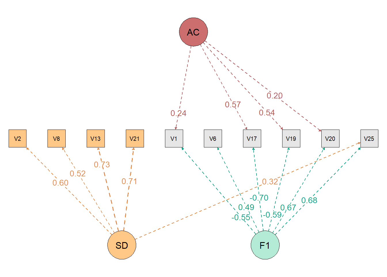
The example contains 10 variables from 300 respondents. Four variables are desirability markers, while the remaining six represent physical aggression. The content items include positively and negatively keyed indicators.
DETAILS OF ANALYSIS

Number of participants                      :   300
Number of items                             :    10
Items selected as SD items                  :  1, 2, 3, 4
Items selected as unbalanced                :  0
Dispersion Matrix                           : Polychoric Correlations
Method for factor extraction                : Unweighted Least Squares (ULS)
Rotation Method                             : none

-----------------------------------------------------------------------

Univariate item descriptives

Item       Mean        Variance    Skewness     Kurtosis (Zero centered)

Item   1   3.667       1.260      -0.555       -0.566
Item   2   3.263       1.760      -0.379       -1.005
Item   3   2.317       1.695       0.601       -0.880
Item   4   2.947       1.924      -0.033       -1.284
Item   5   3.643       1.374      -0.565       -0.535
Item   6   2.467       1.802       0.487       -0.967
Item   7   3.710       1.678      -0.652       -0.716
Item   8   3.493       1.629      -0.411       -0.862
Item   9   1.997       1.515       1.041       -0.011
Item  10   1.687       0.925       1.293        0.838

Polychoric correlation is advised when the univariate distributions of ordinal items are
asymmetric or with excess of kurtosis. If both indices are lower than one in absolute value,
then Pearson correlation is advised. You can read more about this subject in:

Muthen, B., & Kaplan D. (1985). A Comparison of Some Methodologies for the Factor Analysis of
Non-Normal Likert Variables. British Journal of Mathematical and Statistical Psychology, 38, 171-189.

Muthen, B., & Kaplan D. (1992). A Comparison of Some Methodologies for the Factor Analysis of
Non-Normal Likert Variables: A Note on the Size of the Model. British Journal of Mathematical
and Statistical Psychology, 45, 19-30.

-----------------------------------------------------------------------

Adequacy of the dispersion matrix

Determinant of the matrix     = 0.047816437916936
Bartlett's statistic          =   896.4 (df =    45; P = 0.000000)
Kaiser-Meyer-Olkin (KMO) test = 0.76664 (fair)

-----------------------------------------------------------------------
EXPLORATORY FACTOR ANALYSIS CONTROLLING SOCIAL DESIRABILITY AND ACQUIESCENCE
-----------------------------------------------------------------------

Robust Goodness of Fit statistics

          Root Mean Square Error of Approximation (RMSEA) = 0.032

 Robust Mean-Scaled Chi Square with 23 degrees of freedom = 30.146

              Non-Normed Fit Index (NNFI; Tucker & Lewis) = 0.989
                              Comparative Fit Index (CFI) = 0.994
                              Goodness of Fit Index (GFI) = 0.977

-----------------------------------------------------------------------

                  Root Mean Square Residuals (RMSR) = 0.0452
Expected mean value of RMSR for an acceptable model = 0.0578 (Kelley's criterion)

-----------------------------------------------------------------------

Unrotated loading matrix

         Factor SD Factor AC Factor 1
Item   1   0.60252   0.00000  0.00000
Item   2   0.51526   0.00000  0.00000
Item   3   0.72702   0.00000  0.00000
Item   4   0.71131   0.00000  0.00000
Item   5  -0.07850   0.23751 -0.54832
Item   6   0.27517   0.00263  0.49072
Item   7  -0.16411   0.57387 -0.70155
Item   8  -0.14318   0.54034 -0.59125
Item   9   0.26557   0.19660  0.66828
Item  10   0.31730   0.06258  0.68212
Here, contAC = TRUE requests simultaneous control for acquiescence. If acquiescence is not part of the analysis, change it to FALSE.
The output should be interpreted at three levels:
- the content-factor solution after response-bias components are taken into account;
- loadings associated with the social-desirability and acquiescence components; and
- the adequacy and interpretability of the resulting factor solution.
Factor scores can also be requested:
Computing EAP scores. Time remaining  0 seconds
Computing EAP scores. Time remaining  0 seconds
Computing EAP scores. Time remaining  0 seconds
Computing EAP scores. Time remaining  2 seconds
Computing EAP scores. Time remaining  2 seconds
Computing EAP scores. Time remaining  1 seconds
Computing EAP scores. Time remaining  1 seconds
Computing EAP scores. Time remaining  1 seconds
Computing EAP scores. Time remaining  1 seconds
Computing EAP scores. Time remaining  1 seconds
Computing EAP scores. Time remaining  1 seconds
Computing EAP scores. Time remaining  1 seconds
Computing EAP scores. Time remaining  1 seconds
Computing EAP scores. Time remaining  1 seconds
Computing EAP scores. Time remaining  1 seconds
Computing EAP scores. Time remaining  1 seconds
Computing EAP scores. Time remaining  1 seconds
Computing EAP scores. Time remaining  1 seconds
Computing EAP scores. Time remaining  1 seconds
Computing EAP scores. Time remaining  1 seconds
Computing EAP scores. Time remaining  1 seconds
Computing EAP scores. Time remaining  1 seconds
Computing EAP scores. Time remaining  1 seconds
Computing EAP scores. Time remaining  1 seconds
Computing EAP scores. Time remaining  1 seconds
Computing EAP scores. Time remaining  1 seconds
Computing EAP scores. Time remaining  1 seconds
Computing EAP scores. Time remaining  1 seconds
Computing EAP scores. Time remaining  1 seconds
Computing EAP scores. Time remaining  1 seconds
Computing EAP scores. Time remaining  1 seconds
Computing EAP scores. Time remaining  1 seconds
Computing EAP scores. Time remaining  1 seconds
Computing EAP scores. Time remaining  1 seconds
Computing EAP scores. Time remaining  1 seconds
Computing EAP scores. Time remaining  1 seconds
Computing EAP scores. Time remaining  1 seconds
Computing EAP scores. Time remaining  1 seconds
Computing EAP scores. Time remaining  1 seconds
Computing EAP scores. Time remaining  1 seconds
Computing EAP scores. Time remaining  1 seconds
Computing EAP scores. Time remaining  1 seconds
Computing EAP scores. Time remaining  1 seconds
Computing EAP scores. Time remaining  1 seconds
Computing EAP scores. Time remaining  1 seconds
Computing EAP scores. Time remaining  1 seconds
Computing EAP scores. Time remaining  1 seconds
Computing EAP scores. Time remaining  1 seconds
Computing EAP scores. Time remaining  1 seconds
Computing EAP scores. Time remaining  1 seconds
Computing EAP scores. Time remaining  1 seconds
Computing EAP scores. Time remaining  1 seconds
Computing EAP scores. Time remaining  1 seconds
Computing EAP scores. Time remaining  1 seconds
Computing EAP scores. Time remaining  1 seconds
Computing EAP scores. Time remaining  1 seconds
Computing EAP scores. Time remaining  1 seconds
Computing EAP scores. Time remaining  1 seconds
Computing EAP scores. Time remaining  1 seconds
Computing EAP scores. Time remaining  1 seconds
Computing EAP scores. Time remaining  1 seconds
Computing EAP scores. Time remaining  1 seconds
Computing EAP scores. Time remaining  1 seconds
Computing EAP scores. Time remaining  1 seconds
Computing EAP scores. Time remaining  1 seconds
Computing EAP scores. Time remaining  1 seconds
Computing EAP scores. Time remaining  1 seconds
Computing EAP scores. Time remaining  1 seconds
Computing EAP scores. Time remaining  1 seconds
Computing EAP scores. Time remaining  1 seconds
Computing EAP scores. Time remaining  1 seconds
Computing EAP scores. Time remaining  1 seconds
Computing EAP scores. Time remaining  1 seconds
Computing EAP scores. Time remaining  1 seconds
Computing EAP scores. Time remaining  1 seconds
Computing EAP scores. Time remaining  1 seconds
Computing EAP scores. Time remaining  1 seconds
Computing EAP scores. Time remaining  1 seconds
Computing EAP scores. Time remaining  1 seconds
Computing EAP scores. Time remaining  1 seconds
Computing EAP scores. Time remaining  1 seconds
Computing EAP scores. Time remaining  1 seconds
Computing EAP scores. Time remaining  1 seconds
Computing EAP scores. Time remaining  1 seconds
Computing EAP scores. Time remaining  1 seconds
Computing EAP scores. Time remaining  1 seconds
Computing EAP scores. Time remaining  1 seconds
Computing EAP scores. Time remaining  1 seconds
Computing EAP scores. Time remaining  1 seconds
Computing EAP scores. Time remaining  1 seconds
Computing EAP scores. Time remaining  1 seconds
Computing EAP scores. Time remaining  1 seconds
Computing EAP scores. Time remaining  1 seconds
Computing EAP scores. Time remaining  1 seconds
Computing EAP scores. Time remaining  1 seconds
Computing EAP scores. Time remaining  1 seconds
Computing EAP scores. Time remaining  1 seconds
Computing EAP scores. Time remaining  1 seconds
Computing EAP scores. Time remaining  1 seconds
Computing EAP scores. Time remaining  1 seconds
Computing EAP scores. Time remaining  1 seconds
Computing EAP scores. Time remaining  1 seconds
Computing EAP scores. Time remaining  1 seconds
Computing EAP scores. Time remaining  1 seconds
Computing EAP scores. Time remaining  1 seconds
Computing EAP scores. Time remaining  1 seconds
Computing EAP scores. Time remaining  1 seconds
Computing EAP scores. Time remaining  1 seconds
Computing EAP scores. Time remaining  1 seconds
Computing EAP scores. Time remaining  1 seconds
Computing EAP scores. Time remaining  1 seconds
Computing EAP scores. Time remaining  1 seconds
Computing EAP scores. Time remaining  1 seconds
Computing EAP scores. Time remaining  1 seconds
Computing EAP scores. Time remaining  1 seconds
Computing EAP scores. Time remaining  1 seconds
Computing EAP scores. Time remaining  1 seconds
Computing EAP scores. Time remaining  1 seconds
Computing EAP scores. Time remaining  1 seconds
Computing EAP scores. Time remaining  1 seconds
Computing EAP scores. Time remaining  1 seconds
Computing EAP scores. Time remaining  1 seconds
Computing EAP scores. Time remaining  1 seconds
Computing EAP scores. Time remaining  1 seconds
Computing EAP scores. Time remaining  1 seconds
Computing EAP scores. Time remaining  1 seconds
Computing EAP scores. Time remaining  1 seconds
Computing EAP scores. Time remaining  1 seconds
Computing EAP scores. Time remaining  1 seconds
Computing EAP scores. Time remaining  1 seconds
Computing EAP scores. Time remaining  1 seconds
Computing EAP scores. Time remaining  1 seconds
Computing EAP scores. Time remaining  1 seconds
Computing EAP scores. Time remaining  1 seconds
Computing EAP scores. Time remaining  1 seconds
Computing EAP scores. Time remaining  1 seconds
Computing EAP scores. Time remaining  1 seconds
Computing EAP scores. Time remaining  1 seconds
Computing EAP scores. Time remaining  1 seconds
Computing EAP scores. Time remaining  1 seconds
Computing EAP scores. Time remaining  1 seconds
Computing EAP scores. Time remaining  1 seconds
Computing EAP scores. Time remaining  1 seconds
Computing EAP scores. Time remaining  1 seconds
Computing EAP scores. Time remaining  1 seconds
Computing EAP scores. Time remaining  1 seconds
Computing EAP scores. Time remaining  1 seconds
Computing EAP scores. Time remaining  1 seconds
Computing EAP scores. Time remaining  1 seconds
Computing EAP scores. Time remaining  1 seconds
Computing EAP scores. Time remaining  1 seconds
Computing EAP scores. Time remaining  1 seconds
Computing EAP scores. Time remaining  1 seconds
Computing EAP scores. Time remaining  1 seconds
Computing EAP scores. Time remaining  1 seconds
Computing EAP scores. Time remaining  1 seconds
Computing EAP scores. Time remaining  1 seconds
Computing EAP scores. Time remaining  1 seconds
Computing EAP scores. Time remaining  1 seconds
Computing EAP scores. Time remaining  1 seconds
Computing EAP scores. Time remaining  1 seconds
Computing EAP scores. Time remaining  1 seconds
Computing EAP scores. Time remaining  1 seconds
Computing EAP scores. Time remaining  1 seconds
Computing EAP scores. Time remaining  1 seconds
Computing EAP scores. Time remaining  1 seconds
Computing EAP scores. Time remaining  1 seconds
Computing EAP scores. Time remaining  1 seconds
Computing EAP scores. Time remaining  1 seconds
Computing EAP scores. Time remaining  1 seconds
Computing EAP scores. Time remaining  1 seconds
Computing EAP scores. Time remaining  1 seconds
Computing EAP scores. Time remaining  1 seconds
Computing EAP scores. Time remaining  1 seconds
Computing EAP scores. Time remaining  1 seconds
Computing EAP scores. Time remaining  1 seconds
Computing EAP scores. Time remaining  1 seconds
Computing EAP scores. Time remaining  1 seconds
Computing EAP scores. Time remaining  1 seconds
Computing EAP scores. Time remaining  1 seconds
Computing EAP scores. Time remaining  1 seconds
Computing EAP scores. Time remaining  1 seconds
Computing EAP scores. Time remaining  1 seconds
Computing EAP scores. Time remaining  1 seconds
Computing EAP scores. Time remaining  1 seconds
Computing EAP scores. Time remaining  1 seconds
Computing EAP scores. Time remaining  1 seconds
Computing EAP scores. Time remaining  1 seconds
Computing EAP scores. Time remaining  1 seconds
Computing EAP scores. Time remaining  1 seconds
Computing EAP scores. Time remaining  1 seconds
Computing EAP scores. Time remaining  1 seconds
Computing EAP scores. Time remaining  1 seconds
Computing EAP scores. Time remaining  1 seconds
Computing EAP scores. Time remaining  1 seconds
Computing EAP scores. Time remaining  1 seconds
Computing EAP scores. Time remaining  1 seconds
Computing EAP scores. Time remaining  1 seconds
Computing EAP scores. Time remaining  1 seconds
Computing EAP scores. Time remaining  1 seconds
Computing EAP scores. Time remaining  1 seconds
Computing EAP scores. Time remaining  1 seconds
Computing EAP scores. Time remaining  1 seconds
Computing EAP scores. Time remaining  1 seconds
Computing EAP scores. Time remaining  1 seconds
Computing EAP scores. Time remaining  1 seconds
Computing EAP scores. Time remaining  1 seconds
Computing EAP scores. Time remaining  1 seconds
Computing EAP scores. Time remaining  1 seconds
Computing EAP scores. Time remaining  1 seconds
Computing EAP scores. Time remaining  1 seconds
Computing EAP scores. Time remaining  1 seconds
Computing EAP scores. Time remaining  1 seconds
Computing EAP scores. Time remaining  1 seconds
Computing EAP scores. Time remaining  1 seconds
Computing EAP scores. Time remaining  1 seconds
Computing EAP scores. Time remaining  1 seconds
Computing EAP scores. Time remaining  1 seconds
Computing EAP scores. Time remaining  1 seconds
Computing EAP scores. Time remaining  1 seconds
Computing EAP scores. Time remaining  1 seconds
Computing EAP scores. Time remaining  1 seconds
Computing EAP scores. Time remaining  1 seconds
Computing EAP scores. Time remaining  1 seconds
Computing EAP scores. Time remaining  1 seconds
Computing EAP scores. Time remaining  1 seconds
Computing EAP scores. Time remaining  1 seconds
Computing EAP scores. Time remaining  1 seconds
Computing EAP scores. Time remaining  1 seconds
Computing EAP scores. Time remaining  1 seconds
Computing EAP scores. Time remaining  1 seconds
Computing EAP scores. Time remaining  1 seconds
Computing EAP scores. Time remaining  1 seconds
Computing EAP scores. Time remaining  1 seconds
Computing EAP scores. Time remaining  1 seconds
Computing EAP scores. Time remaining  1 seconds
Computing EAP scores. Time remaining  1 seconds
Computing EAP scores. Time remaining  1 seconds
Computing EAP scores. Time remaining  1 seconds
Computing EAP scores. Time remaining  1 seconds
Computing EAP scores. Time remaining  1 seconds
Computing EAP scores. Time remaining  1 seconds
Computing EAP scores. Time remaining  1 seconds
Computing EAP scores. Time remaining  1 seconds
Computing EAP scores. Time remaining  1 seconds
Computing EAP scores. Time remaining  1 seconds
Computing EAP scores. Time remaining  1 seconds
Computing EAP scores. Time remaining  1 seconds
Computing EAP scores. Time remaining  1 seconds
Computing EAP scores. Time remaining  1 seconds
Computing EAP scores. Time remaining  1 seconds
Computing EAP scores. Time remaining  1 seconds
Computing EAP scores. Time remaining  1 seconds
Computing EAP scores. Time remaining  1 seconds
Computing EAP scores. Time remaining  1 seconds
Computing EAP scores. Time remaining  1 seconds
Computing EAP scores. Time remaining  1 seconds
Computing EAP scores. Time remaining  1 seconds
Computing EAP scores. Time remaining  1 seconds
Computing EAP scores. Time remaining  1 seconds
Computing EAP scores. Time remaining  1 seconds
Computing EAP scores. Time remaining  1 seconds
Computing EAP scores. Time remaining  1 seconds
Computing EAP scores. Time remaining  1 seconds
Computing EAP scores. Time remaining  1 seconds
Computing EAP scores. Time remaining  1 seconds
Computing EAP scores. Time remaining  1 seconds
Computing EAP scores. Time remaining  1 seconds
Computing EAP scores. Time remaining  1 seconds
Computing EAP scores. Time remaining  1 seconds
Computing EAP scores. Time remaining  1 seconds
Computing EAP scores. Time remaining  1 seconds
Computing EAP scores. Time remaining  1 seconds
Computing EAP scores. Time remaining  1 seconds
Computing EAP scores. Time remaining  1 seconds
Computing EAP scores. Time remaining  1 seconds
Computing EAP scores. Time remaining  1 seconds
Computing EAP scores. Time remaining  1 seconds
Computing EAP scores. Time remaining  1 seconds
Computing EAP scores. Time remaining  1 seconds
Computing EAP scores. Time remaining  1 seconds
Computing EAP scores. Time remaining  1 seconds
Computing EAP scores. Time remaining  1 seconds
Computing EAP scores. Time remaining  1 seconds
Computing EAP scores. Time remaining  1 seconds
Computing EAP scores. Time remaining  1 seconds
Computing EAP scores. Time remaining  1 seconds
Computing EAP scores. Time remaining  1 seconds
Computing EAP scores. Time remaining  1 seconds
Computing EAP scores. Time remaining  1 seconds
Computing EAP scores. Time remaining  1 seconds
Computing EAP scores. Time remaining  1 seconds
Computing EAP scores. Time remaining  1 seconds
Computing EAP scores. Time remaining  1 seconds
Computing EAP scores. Time remaining  1 seconds
Computing EAP scores. Time remaining  1 seconds
Computing EAP scores. Time remaining  1 seconds
Computing EAP scores. Time remaining  1 seconds
Computing EAP scores. Time remaining  1 seconds
Computing EAP scores. Time remaining  0 seconds


DETAILS OF ANALYSIS

Number of participants                      :   300
Number of items                             :    10
Items selected as SD items                  :  1, 2, 3, 4
Items selected as unbalanced                :  0
Dispersion Matrix                           : Polychoric Correlations
Method for factor extraction                : Unweighted Least Squares (ULS)
Rotation Method                             : none

-----------------------------------------------------------------------

Univariate item descriptives

Item       Mean        Variance    Skewness     Kurtosis (Zero centered)

Item   1   3.667       1.260      -0.555       -0.566
Item   2   3.263       1.760      -0.379       -1.005
Item   3   2.317       1.695       0.601       -0.880
Item   4   2.947       1.924      -0.033       -1.284
Item   5   3.643       1.374      -0.565       -0.535
Item   6   2.467       1.802       0.487       -0.967
Item   7   3.710       1.678      -0.652       -0.716
Item   8   3.493       1.629      -0.411       -0.862
Item   9   1.997       1.515       1.041       -0.011
Item  10   1.687       0.925       1.293        0.838

Polychoric correlation is advised when the univariate distributions of ordinal items are
asymmetric or with excess of kurtosis. If both indices are lower than one in absolute value,
then Pearson correlation is advised. You can read more about this subject in:

Muthen, B., & Kaplan D. (1985). A Comparison of Some Methodologies for the Factor Analysis of
Non-Normal Likert Variables. British Journal of Mathematical and Statistical Psychology, 38, 171-189.

Muthen, B., & Kaplan D. (1992). A Comparison of Some Methodologies for the Factor Analysis of
Non-Normal Likert Variables: A Note on the Size of the Model. British Journal of Mathematical
and Statistical Psychology, 45, 19-30.

-----------------------------------------------------------------------

Adequacy of the dispersion matrix

Determinant of the matrix     = 0.047816437916936
Bartlett's statistic          =   896.4 (df =    45; P = 0.000000)
Kaiser-Meyer-Olkin (KMO) test = 0.76664 (fair)

-----------------------------------------------------------------------
EXPLORATORY FACTOR ANALYSIS CONTROLLING SOCIAL DESIRABILITY AND ACQUIESCENCE
-----------------------------------------------------------------------

Robust Goodness of Fit statistics

          Root Mean Square Error of Approximation (RMSEA) = 0.032

 Robust Mean-Scaled Chi Square with 23 degrees of freedom = 30.146

              Non-Normed Fit Index (NNFI; Tucker & Lewis) = 0.989
                              Comparative Fit Index (CFI) = 0.994
                              Goodness of Fit Index (GFI) = 0.977

-----------------------------------------------------------------------

                  Root Mean Square Residuals (RMSR) = 0.0452
Expected mean value of RMSR for an acceptable model = 0.0578 (Kelley's criterion)

-----------------------------------------------------------------------

Unrotated loading matrix

         Factor SD Factor AC Factor 1
Item   1   0.60257   0.00000  0.00000
Item   2   0.51525   0.00000  0.00000
Item   3   0.72709   0.00000  0.00000
Item   4   0.71129   0.00000  0.00000
Item   5  -0.07851   0.23762 -0.54830
Item   6   0.27519   0.00217  0.49050
Item   7  -0.16412   0.57419 -0.70137
Item   8  -0.14320   0.54067 -0.59104
Item   9   0.26559   0.19597  0.66799
Item  10   0.31732   0.06246  0.68221

-----------------------------------------------------------------------

RELIABILITY OF EAP SCORES

Factor         EAP Reliability estimate

SD           :  0.6741
Acquiescence :  0.4110
Factor 1     :  0.6589

PARTICIPANTS'S SCORES ON FACTORS:
Rescaled to mean = 50 and standard deviation = 10 in the sample

       Factor SD Factor AC Factor 1
  [1,]  44.30701  48.53108 48.55202
  [2,]  59.62138  38.14741 49.43079
  [3,]  61.18625  42.28635 42.33527
  [4,]  55.02636  43.35037 43.33025
  [5,]  48.22922  38.64151 60.28440
  [6,]  44.51591  64.27684 45.87749
  [7,]  44.73255  65.04926 56.23803
  [8,]  39.63917  50.43811 71.99098
  [9,]  61.34344  36.08764 45.46285
 [10,]  52.16717  54.33677 54.70079
 [11,]  55.76827  44.66385 56.05595
 [12,]  53.40486  58.26886 58.40459
 [13,]  46.67115  51.21173 51.35699
 [14,]  78.49690  78.23462 55.24198
 [15,]  55.73240  54.95498 55.71045
 [16,]  44.79377  64.48834 37.53640
 [17,]  45.01397  46.08958 56.32517
 [18,]  44.88619  59.48709 55.32836
 [19,]  43.98181  35.51016 67.03736
 [20,]  56.02792  34.92565 54.53968
 [21,]  43.26937  33.50092 43.18549
 [22,]  55.84771  64.01367 66.76828
 [23,]  28.12220  58.07185 33.26633
 [24,]  49.33772  42.43312 50.63642
 [25,]  39.89137  45.29797 47.25504
 [26,]  37.03565  57.53473 42.78019
 [27,]  55.01197  47.35786 47.47995
 [28,]  55.91160  62.54166 50.80955
 [29,]  43.96945  45.20953 56.56501
 [30,]  55.62014  44.38368 55.72272
 [31,]  37.85532  65.93751 41.52338
 [32,]  44.88456  43.34268 45.22780
 [33,]  46.71661  40.35834 62.79386
 [34,]  65.13218  49.65353 49.86109
 [35,]  47.81878  48.87813 50.87092
 [36,]  67.06675  41.07778 40.17719
 [37,]  44.91480  53.52407 53.52993
 [38,]  54.25462  57.87583 67.98566
 [39,]  55.62406  44.10900 56.01380
 [40,]  43.18239  54.50944 56.11575
 [41,]  52.53007  46.39364 58.65074
 [42,]  64.91130  50.83205 48.65427
 [43,]  65.34185  53.50412 42.94909
 [44,]  54.85252  42.88793 54.41311
 [45,]  55.73982  55.70866 55.73461
 [46,]  52.50584  44.32355 55.29879
 [47,]  34.77558  41.69290 52.74273
 [48,]  45.26303  45.00804 56.26994
 [49,]  32.23582  36.27421 50.71474
 [50,]  55.73954  43.90114 44.00651
 [51,]  32.22493  56.28736 56.28759
 [52,]  49.72712  51.33979 41.26882
 [53,]  46.28992  38.95460 51.22886
 [54,]  50.74997  58.68553 30.04858
 [55,]  56.36378  50.67707 67.06379
 [56,]  34.49170  41.64022 38.07818
 [57,]  44.14537  50.13263 45.75367
 [58,]  44.05198  53.41548 53.43084
 [59,]  78.32488  61.79794 45.64526
 [60,]  46.94949  53.90589 54.39186
 [61,]  78.53937  71.24588 43.46483
 [62,]  55.64334  47.45841 55.71923
 [63,]  43.98731  53.49975 55.68979
 [64,]  57.69312  47.71475 64.03548
 [65,]  55.68321  42.58519 53.78265
 [66,]  55.60386  43.40730 55.72978
 [67,]  55.75809  56.92097 56.40342
 [68,]  64.71213  52.12510 56.32229
 [69,]  45.40363  60.13967 33.71294
 [70,]  48.54707  62.54332 37.06513
 [71,]  43.40332  44.68100 45.23626
 [72,]  43.79681  58.55066 31.07520
 [73,]  37.82992  58.37995 31.92960
 [74,]  72.68739  68.25381 40.04592
 [75,]  38.54145  60.71585 46.16882
 [76,]  44.39734  77.52058 66.33631
 [77,]  34.98962  43.00002 66.00357
 [78,]  42.29032  37.14529 47.71327
 [79,]  55.43490  33.82119 64.89849
 [80,]  41.19005  67.25730 43.43257
 [81,]  44.31976  50.67432 55.39842
 [82,]  78.46787  61.62999 30.43687
 [83,]  53.24780  71.49634 72.34327
 [84,]  41.17021  50.35090 43.28430
 [85,]  55.38927  62.00664 61.94293
 [86,]  44.96839  74.33731 78.48550
 [87,]  54.44504  39.63063 67.51161
 [88,]  51.48323  52.16362 45.84701
 [89,]  45.36002  43.61214 59.94967
 [90,]  55.82145  45.90406 45.89933
 [91,]  37.66105  71.90680 48.64857
 [92,]  44.12224  53.92678 53.94084
 [93,]  34.83375  66.23422 61.57234
 [94,]  54.82501  53.86442 54.17176
 [95,]  66.64026  51.15448 39.68492
 [96,]  67.81858  78.46801 55.73766
 [97,]  56.12518  51.65467 55.46954
 [98,]  33.52509  58.25343 32.54090
 [99,]  48.00185  51.29224 44.86860
[100,]  54.34950  53.19997 56.70573
[101,]  44.91288  68.09801 44.32200
[102,]  66.49211  44.36762 56.00912
[103,]  49.86799  66.59253 50.03713
[104,]  44.95695  65.11863 67.23711
[105,]  33.06385  48.68058 50.14241
[106,]  75.49482  42.91828 46.03487
[107,]  56.44246  55.56866 65.95981
[108,]  70.56547  54.84812 53.73933
[109,]  56.47425  66.36626 47.59875
[110,]  54.43004  50.10789 59.49633
[111,]  44.33457  46.82482 46.59368
[112,]  55.87862  50.68531 50.67717
[113,]  40.23216  46.74074 46.49343
[114,]  60.99477  46.11130 44.07640
[115,]  55.65058  34.95109 54.73447
[116,]  66.93588  44.63601 43.63745
[117,]  55.99766  56.98890 57.68375
[118,]  55.54200  58.41736 58.53135
[119,]  44.58476  49.91317 49.93617
[120,]  75.70628  57.32543 33.60860
[121,]  53.27321  48.43855 48.43924
[122,]  46.07408  37.19317 55.68566
[123,]  67.24767  55.06490 55.28679
[124,]  38.76287  50.00618 55.43151
[125,]  64.49811  52.49385 52.50490
[126,]  41.73244  58.49105 31.37057
[127,]  43.14170  46.41235 77.99035
[128,]  41.30294  45.13437 67.11730
[129,]  42.51574  62.30447 43.75108
[130,]  31.75776  35.56369 47.12999
[131,]  37.36628  75.93414 66.44332
[132,]  46.14688  58.59219 30.72566
[133,]  43.81891  41.37265 52.70027
[134,]  66.99872  55.76471 57.00761
[135,]  44.32075  36.68566 67.10887
[136,]  42.22617  58.50578 31.30020
[137,]  43.89432  48.57712 48.73682
[138,]  65.19128  49.37094 37.87734
[139,]  42.66219  71.28397 56.58937
[140,]  33.86136  58.26464 32.49538
[141,]  42.68994  46.67950 36.45908
[142,]  44.93871  52.98705 42.23349
[143,]  55.74581  46.76498 55.17295
[144,]  49.67967  58.66335 30.20444
[145,]  32.17281  47.61256 56.68694
[146,]  47.70305  40.14519 40.12169
[147,]  29.64896  58.02735 45.31533
[148,]  33.28932  40.06241 53.67718
[149,]  55.81780  46.34863 57.66354
[150,]  48.66224  58.64674 30.35768
[151,]  47.97415  55.06853 56.18060
[152,]  43.65891  38.22845 61.94341
[153,]  54.17812  46.08165 57.77608
[154,]  61.57328  49.03333 37.04562
[155,]  43.33181  58.53729 31.14177
[156,]  55.71442  58.77401 29.30729
[157,]  53.68776  55.24015 55.22009
[158,]  44.74144  57.76006 41.50823
[159,]  55.04712  47.06459 50.58313
[160,]  44.81192  58.57472 30.92741
[161,]  55.75063  63.31866 43.50675
[162,]  60.59029  46.32817 45.30926
[163,]  68.79728  42.98774 42.84378
[164,]  56.44139  64.91748 64.83057
[165,]  43.76941  43.79634 42.24331
[166,]  55.74944  52.56716 55.52064
[167,]  55.72438  45.39506 55.63701
[168,]  55.67130  49.90725 51.34229
[169,]  56.73583  68.11540 42.76953
[170,]  68.26755  40.71651 46.55638
[171,]  62.50534  67.15730 39.97988
[172,]  53.84667  47.51465 48.21877
[173,]  67.01734  55.69224 55.57967
[174,]  42.47363  57.66482 41.61226
[175,]  67.06214  47.50433 55.69087
[176,]  50.89323  63.06702 52.59677
[177,]  46.05382  60.55515 44.43494
[178,]  54.32947  55.21161 44.13109
[179,]  56.59253  46.35268 44.10420
[180,]  44.87849  49.54493 38.59122
[181,]  58.31664  44.61238 44.32336
[182,]  54.62445  47.85768 48.69596
[183,]  60.12665  58.57206 55.69575
[184,]  34.35325  58.27920 32.42570
[185,]  47.21502  58.61982 30.57190
[186,]  60.62144  46.21341 34.25969
[187,]  78.42770  58.70180 34.76222
[188,]  37.86695  57.55925 42.64818
[189,]  55.41232  42.21178 54.81368
[190,]  47.63988  54.35476 64.35083
[191,]  55.69734  44.73767 44.72971
[192,]  62.74632  44.58665 46.68503
[193,]  41.00049  49.14216 39.38732
[194,]  56.91885  47.76392 76.15910
[195,]  41.66044  40.41011 68.90212
[196,]  55.68583  39.83030 55.11935
[197,]  68.74465  61.61819 55.83638
[198,]  55.57550  56.17652 44.81807
[199,]  55.71430  69.79323 41.83343
[200,]  44.21235  56.42914 56.46142
[201,]  55.18636  47.82623 56.76818
[202,]  44.77243  69.69359 46.28913
[203,]  51.10428  41.49555 47.76118
[204,]  56.46256  77.80215 55.65609
[205,]  39.54438  60.63929 45.90737
[206,]  44.14108  60.14961 33.95550
[207,]  61.72461  43.41597 55.69178
[208,]  54.38081  46.29163 66.08591
[209,]  50.23607  46.52342 46.56268
[210,]  44.67939  48.55557 43.72594
[211,]  58.58177  57.01626 65.11569
[212,]  55.73808  58.77796 29.30964
[213,]  54.03617  32.77291 53.46468
[214,]  55.87395  58.77757 29.28467
[215,]  41.35666  50.67146 50.24655
[216,]  47.10619  52.42834 74.55462
[217,]  50.97880  67.98246 42.35222
[218,]  55.74765  51.41262 42.28641
[219,]  58.51372  43.21230 67.12063
[220,]  51.74153  42.13171 45.85932
[221,]  77.23746  50.45728 78.38560
[222,]  55.68603  66.10306 44.69160
[223,]  45.46759  48.19078 48.15096
[224,]  29.00415  62.70807 47.09119
[225,]  67.09954  44.87643 44.67446
[226,]  44.36776  66.29706 67.22509
[227,]  39.95165  36.14293 58.53979
[228,]  56.17736  36.70008 44.14978
[229,]  45.74829  60.13696 33.64622
[230,]  67.13420  46.00472 45.95450
[231,]  44.94890  55.42788 55.56346
[232,]  55.60048  44.88343 44.95203
[233,]  55.71750  43.85535 55.71209
[234,]  67.10077  44.62075 44.58494
[235,]  67.23646  35.23233 46.58278
[236,]  48.49785  58.64362 30.38196
[237,]  55.69186  44.54974 44.54204
[238,]  43.46603  45.45763 36.05378
[239,]  43.86774  33.04188 44.11042
[240,]  66.99800  44.58227 44.52703
[241,]  56.14267  44.02456 55.15464
[242,]  61.02502  38.24302 45.62884
[243,]  42.85201  51.89690 64.26466
[244,]  55.70343  59.37584 47.98454
[245,]  55.73565  55.37287 44.02408
[246,]  58.90467  58.04529 37.69489
[247,]  55.73357  44.57461 56.41493
[248,]  44.26878  38.82406 52.68050
[249,]  36.53861  75.31109 51.80845
[250,]  78.49793  54.79512 44.19334
[251,]  65.90953  45.74340 75.74219
[252,]  55.80844  44.30286 55.23457
[253,]  71.61781  44.53133 32.26731
[254,]  70.39185  51.52310 53.04271
[255,]  66.84941  36.94742 67.05290
[256,]  66.65350  60.65353 49.67673
[257,]  45.58459  45.56319 35.66377
[258,]  55.70545  47.17249 50.33604
[259,]  48.96286  51.77813 52.40321
[260,]  75.67159  46.46903 46.04864
[261,]  45.70171  46.84214 35.91939
[262,]  51.98463  43.83745 43.83529
[263,]  55.51929  71.16138 43.94496
[264,]  34.67687  29.94087 46.18497
[265,]  44.45839  67.56616 43.65206
[266,]  41.74766  58.49198 31.36866
[267,]  33.97261  58.64133 44.63196
[268,]  50.61057  58.91399 51.48937
[269,]  35.30987  63.30393 39.73258
[270,]  34.33509  34.58958 68.97580
[271,]  53.11267  42.91709 45.88642
[272,]  67.40973  45.39324 55.76110
[273,]  53.08524  60.07884 32.25711
[274,]  55.68584  72.87877 54.23249
[275,]  55.47554  57.60425 46.24301
[276,]  45.34846  58.58506 30.84816
[277,]  37.00517  70.17388 55.61616
[278,]  40.28614  53.76325 55.37406
[279,]  44.44572  56.11214 67.36096
[280,]  45.25826  59.73420 50.73335
[281,]  55.31350  60.06111 31.83511
[282,]  44.27975  62.83794 38.28146
[283,]  55.54177  47.69208 66.12952
[284,]  55.28961  38.82365 57.40962
[285,]  51.52534  58.69948 29.93308
[286,]  43.30860  57.66488 41.45712
[287,]  67.66624  69.66626 56.13217
[288,]  54.75810  65.92594 46.60027
[289,]  46.98766  37.41970 49.88570
[290,]  55.54859  44.00506 55.56584
[291,]  45.58112  46.66336 55.23592
[292,]  62.80624  55.73447 43.75547
[293,]  45.74769  51.33571 51.41575
[294,]  52.38584  44.70768 34.71360
[295,]  57.57734  50.81225 52.64297
[296,]  75.39585  65.89203 37.66219
[297,]  67.16580  45.44132 55.99977
[298,]  58.57378  36.37319 46.69537
[299,]  55.86659  42.67761 44.49157
[300,]  73.41784  45.75003 57.08362

NOTE: The precision matrices for the  3 factors were not printed for preventing console spacing issues.
These matrices are stored in $Precision_matrix in the output variable.The resulting scores are not bias-free observed traits. They are estimates conditional on the response-bias model and its assumptions, including the treatment of the desirability markers.
9.2 MIMIC Modeling with Peabody Quadruplets
The second example follows the MIMIC-quadruplet logic evaluated by Degobi & Valentini (2023). We use lavaan (Rosseel, 2012) for model simulation and estimation and semPlot (Epskamp, 2022) for a path diagram.
This is lavaan 0.7-2
lavaan is FREE software! Please report any bugs.9.2.1 1. Simulate a design with quadruplets
The following code creates two substantive factors, a social-desirability factor identified by 16 quadruplet items, and 10 additional items whose responses are also influenced by social desirability.
Show data-simulation code
#Quadruple Factor Loadings on Social Desirability
FactorLoadingsSDQ<- rep(0.3, 16)*c(1,-1,1,-1)

#Quadruple Factor Loadings on the Target Construct
RandomFactorLoadingsQ<-rep(0.7, 16)*c(-1,-1,1,1)

# Factor Loads of the extra item in the Target Construct
set.seed(2021)
RandomFactorLoadings <- round(runif((10), min = .3, max = .8), 3)

# Desirability Regressions for Target Construct items
set.seed(2021)
RandomSDregression <- round(runif((10), min = .1, max = .5), 3)

# Item Thresholds
set.seed(2020)
thld1Vet<-round(runif(26, min=-2, max=.5),3)
thld2Vet<-round(thld1Vet +.5,3)
thld3Vet<-round(thld1Vet + 1,3)
thld4Vet<-round(thld1Vet + 1.5,3)

# Simulated Model
simModel <- paste0("fator1 =~",RandomFactorLoadings[1],"*it1 +",
                         RandomFactorLoadings[2],"*it2 +",
                         RandomFactorLoadings[3],"*it3 +",
                         RandomFactorLoadings[4],"*it4 +",
                         RandomFactorLoadings[5],"*it5 +",
                         RandomFactorLoadingsQ[1],"*sd1 +",
                         RandomFactorLoadingsQ[2],"*sd2 +",
                         RandomFactorLoadingsQ[3],"*sd3 +",
                         RandomFactorLoadingsQ[4],"*sd4 +",
                         RandomFactorLoadingsQ[5],"*sd5 +",
                         RandomFactorLoadingsQ[6],"*sd6 +",
                         RandomFactorLoadingsQ[7],"*sd7 +",
                         RandomFactorLoadingsQ[8],"*sd8\n",

                         "fator2 =~", RandomFactorLoadingsQ[6],"*it6 +",
                         RandomFactorLoadingsQ[7],"*it7 +",
                         RandomFactorLoadingsQ[8],"*it8 +",
                         RandomFactorLoadingsQ[9],"*it9 +",
                         RandomFactorLoadingsQ[10],"*it10 +",
                         RandomFactorLoadingsQ[9],"*sd9 +",
                         RandomFactorLoadingsQ[10],"*sd10 +",
                         RandomFactorLoadingsQ[11],"*sd11 +",
                         RandomFactorLoadingsQ[12],"*sd12 +",
                         RandomFactorLoadingsQ[13],"*sd13 +",
                         RandomFactorLoadingsQ[14],"*sd14 +",
                         RandomFactorLoadingsQ[15],"*sd15 +",
                         RandomFactorLoadingsQ[16],"*sd16\n",

                         "SD =~", FactorLoadingsSDQ[1], "*sd1 +",
                         FactorLoadingsSDQ[2],"*sd2 +",
                         FactorLoadingsSDQ[3],"*sd3 +",
                         FactorLoadingsSDQ[4],"*sd4 +",
                         FactorLoadingsSDQ[5], "*sd5 +",
                         FactorLoadingsSDQ[6],"*sd6 +",
                         FactorLoadingsSDQ[7],"*sd7 +",
                         FactorLoadingsSDQ[8],"*sd8 +",
                         FactorLoadingsSDQ[9], "*sd9 +",
                         FactorLoadingsSDQ[10],"*sd10 +",
                         FactorLoadingsSDQ[11],"*sd11 +",
                         FactorLoadingsSDQ[12],"*sd12 +",
                         FactorLoadingsSDQ[13], "*sd13 +",
                         FactorLoadingsSDQ[14],"*sd14 +",
                         FactorLoadingsSDQ[15],"*sd15 +",
                         FactorLoadingsSDQ[16],"*sd16\n",

                         "SD ~~ 1*SD\n",
                         "fator1 ~~ 1*fator1\n",
                         "fator2 ~~ 1*fator2\n",
                         "fator1 ~~ 0*SD\n",
                         "fator2 ~~ 0*SD\n",
                         "fator1 ~~ .3*fator2\n",

                         "it1 ~",RandomSDregression[1],"*SD\n",
                         "it2 ~",RandomSDregression[2],"*SD\n",
                         "it3 ~",RandomSDregression[3],"*SD\n",
                         "it4 ~",RandomSDregression[4],"*SD\n",
                         "it5 ~",RandomSDregression[5],"*SD\n",
                         "it6 ~",RandomSDregression[6],"*SD\n",
                         "it7 ~",RandomSDregression[7],"*SD\n",
                         "it8 ~",RandomSDregression[8],"*SD\n",
                         "it9 ~",RandomSDregression[9],"*SD\n",
                         "it10 ~",RandomSDregression[10],"*SD\n",

                         "sd1 |",thld1Vet[1],"*t1 +", thld2Vet[1], "*t2 +",
                         thld3Vet[1],"*t3 +",thld4Vet[1],"*t4\n",
                         "sd2 |",thld1Vet[2],"*t1 +", thld2Vet[2], "*t2 +",
                         thld3Vet[2],"*t3 +",thld4Vet[2],"*t4\n",
                        "sd3 |",thld1Vet[3],"*t1 +", thld2Vet[3], "*t2 +",
                        thld3Vet[3],"*t3 +",thld4Vet[3],"*t4\n",
                        "sd4 |",thld1Vet[4],"*t1 +", thld2Vet[4], "*t2 +",
                        thld3Vet[4],"*t3 +",thld4Vet[4],"*t4\n",
                        "it1 |",thld1Vet[5],"*t1 +", thld2Vet[5], "*t2 +",
                        thld3Vet[5],"*t3 +",thld4Vet[5],"*t4\n",
                        "it2 |",thld1Vet[6],"*t1 +", thld2Vet[6], "*t2 +",
                        thld3Vet[6],"*t3 +",thld4Vet[6],"*t4\n",
                        "it3 |",thld1Vet[7],"*t1 +", thld2Vet[7], "*t2 +",
                        thld3Vet[7],"*t3 +",thld4Vet[7],"*t4\n",
                        "it4 |",thld1Vet[8],"*t1 +", thld2Vet[8], "*t2 +",
                        thld3Vet[8],"*t3 +",thld4Vet[8],"*t4\n",
                        "it5 |",thld1Vet[9],"*t1 +", thld2Vet[9], "*t2 +",
                        thld3Vet[9],"*t3 +",thld4Vet[9],"*t4\n",
                        "it6 |",thld1Vet[10],"*t1 +", thld2Vet[10], "*t2 +",
                        thld3Vet[10],"*t3 +",thld4Vet[10],"*t4\n",
                        "it7 |",thld1Vet[11],"*t1 +", thld2Vet[11], "*t2 +",
                        thld3Vet[11],"*t3 +",thld4Vet[11],"*t4\n",
                        "it8 |",thld1Vet[12],"*t1 +", thld2Vet[12], "*t2 +",
                        thld3Vet[12],"*t3 +",thld4Vet[12],"*t4\n",
                        "it9 |",thld1Vet[13],"*t1 +", thld2Vet[13], "*t2 +",
                        thld3Vet[13],"*t3 +",thld4Vet[13],"*t4\n",
                        "it10 |",thld1Vet[14],"*t1 +", thld2Vet[14], "*t2 +",
                        thld3Vet[14],"*t3 +",thld4Vet[14],"*t4\n",
                        "sd5 |",thld1Vet[15],"*t1 +", thld2Vet[15], "*t2 +",
                        thld3Vet[15],"*t3 +",thld4Vet[15],"*t4\n",
                        "sd6 |",thld1Vet[16],"*t1 +", thld2Vet[16], "*t2 +",
                        thld3Vet[16],"*t3 +",thld4Vet[16],"*t4\n",
                        "sd7 |",thld1Vet[17],"*t1 +", thld2Vet[17], "*t2 +",
                        thld3Vet[17],"*t3 +",thld4Vet[17],"*t4\n",
                        "sd8 |",thld1Vet[18],"*t1 +", thld2Vet[18], "*t2 +",
                        thld3Vet[18],"*t3 +",thld4Vet[18],"*t4\n",
                        "sd9 |",thld1Vet[19],"*t1 +", thld2Vet[19], "*t2 +",
                        thld3Vet[19],"*t3 +",thld4Vet[19],"*t4\n",
                        "sd10 |",thld1Vet[20],"*t1 +", thld2Vet[20], "*t2 +",
                        thld3Vet[20],"*t3 +",thld4Vet[20],"*t4\n",
                        "sd11 |",thld1Vet[21],"*t1 +", thld2Vet[21], "*t2 +",
                        thld3Vet[21],"*t3 +",thld4Vet[21],"*t4\n",
                        "sd12 |",thld1Vet[22],"*t1 +", thld2Vet[22], "*t2 +",
                        thld3Vet[22],"*t3 +",thld4Vet[22],"*t4\n",
                        "sd13 |",thld1Vet[23],"*t1 +", thld2Vet[23], "*t2 +",
                        thld3Vet[23],"*t3 +",thld4Vet[23],"*t4\n",
                        "sd14 |",thld1Vet[24],"*t1 +", thld2Vet[24], "*t2 +",
                        thld3Vet[24],"*t3 +",thld4Vet[24],"*t4\n",
                        "sd15 |",thld1Vet[25],"*t1 +", thld2Vet[25], "*t2 +",
                        thld3Vet[25],"*t3 +",thld4Vet[25],"*t4\n",
                        "sd16 |",thld1Vet[26],"*t1 +", thld2Vet[26], "*t2 +",
                        thld3Vet[26],"*t3 +",thld4Vet[26],"*t4")

#Simulating the Data
simulatedData <- lavaan::simulateData(model = simModel,
                                       model.type = "sem",
                                       sample.nobs = 4000,
                                       seed = 2024,
                                       return.type = "data.frame",
                                       standardized = TRUE
                                       )
The simulated dataset contains 26 five-category items: 16 items arranged as four quadruplets and 10 additional items outside the quadruplet format.
      it1             it2             it3             it4
 Min.   :1.000   Min.   :1.000   Min.   :1.000   Min.   :1.000
 1st Qu.:3.000   1st Qu.:4.000   1st Qu.:4.000   1st Qu.:2.000
 Median :5.000   Median :5.000   Median :5.000   Median :4.000
 Mean   :4.142   Mean   :4.297   Mean   :4.151   Mean   :3.356
 3rd Qu.:5.000   3rd Qu.:5.000   3rd Qu.:5.000   3rd Qu.:5.000
 Max.   :5.000   Max.   :5.000   Max.   :5.000   Max.   :5.000
      it5             sd1             sd2             sd3
 Min.   :1.000   Min.   :1.000   Min.   :1.000   Min.   :1.000
 1st Qu.:4.000   1st Qu.:1.000   1st Qu.:2.000   1st Qu.:1.000
 Median :5.000   Median :2.000   Median :4.000   Median :2.000
 Mean   :4.436   Mean   :2.507   Mean   :3.344   Mean   :2.606
 3rd Qu.:5.000   3rd Qu.:4.000   3rd Qu.:5.000   3rd Qu.:4.000
 Max.   :5.000   Max.   :5.000   Max.   :5.000   Max.   :5.000
      sd4             sd5            sd6             sd7             sd8
 Min.   :1.000   Min.   :1.00   Min.   :1.000   Min.   :1.000   Min.   :1.000
 1st Qu.:2.000   1st Qu.:2.00   1st Qu.:1.000   1st Qu.:1.000   1st Qu.:1.000
 Median :3.000   Median :3.00   Median :3.000   Median :1.000   Median :2.000
 Mean   :3.082   Mean   :3.31   Mean   :2.857   Mean   :1.639   Mean   :2.485
 3rd Qu.:4.000   3rd Qu.:5.00   3rd Qu.:4.000   3rd Qu.:2.000   3rd Qu.:4.000
 Max.   :5.000   Max.   :5.00   Max.   :5.000   Max.   :5.000   Max.   :5.000
      it6             it7             it8             it9             it10
 Min.   :1.000   Min.   :1.000   Min.   :1.000   Min.   :1.000   Min.   :1.00
 1st Qu.:1.000   1st Qu.:1.000   1st Qu.:1.000   1st Qu.:1.000   1st Qu.:2.00
 Median :2.000   Median :2.000   Median :2.000   Median :1.000   Median :3.00
 Mean   :2.589   Mean   :2.133   Mean   :2.196   Mean   :1.961   Mean   :3.26
 3rd Qu.:4.000   3rd Qu.:3.000   3rd Qu.:3.000   3rd Qu.:3.000   3rd Qu.:5.00
 Max.   :5.000   Max.   :5.000   Max.   :5.000   Max.   :5.000   Max.   :5.00
      sd9             sd10            sd11            sd12
 Min.   :1.000   Min.   :1.000   Min.   :1.000   Min.   :1.000
 1st Qu.:1.000   1st Qu.:3.000   1st Qu.:3.000   1st Qu.:4.000
 Median :3.000   Median :4.000   Median :5.000   Median :5.000
 Mean   :2.835   Mean   :3.772   Mean   :3.957   Mean   :4.281
 3rd Qu.:4.000   3rd Qu.:5.000   3rd Qu.:5.000   3rd Qu.:5.000
 Max.   :5.000   Max.   :5.000   Max.   :5.000   Max.   :5.000
      sd13            sd14            sd15            sd16
 Min.   :1.000   Min.   :1.000   Min.   :1.000   Min.   :1.000
 1st Qu.:1.000   1st Qu.:1.000   1st Qu.:1.000   1st Qu.:3.000
 Median :1.000   Median :1.000   Median :1.000   Median :5.000
 Mean   :1.982   Mean   :1.679   Mean   :1.813   Mean   :4.061
 3rd Qu.:3.000   3rd Qu.:2.000   3rd Qu.:2.000   3rd Qu.:5.000
 Max.   :5.000   Max.   :5.000   Max.   :5.000   Max.   :5.000
9.2.2 2. Specify the empirical MIMIC model
All content-relevant items define their substantive factor. The desirability factor is identified only by the manipulated quadruplet items, and the additional items are regressed on that desirability factor.
The substantive factors are constrained to be orthogonal to the desirability factor for identification in this demonstration. That constraint is a modeling assumption and should be considered carefully in empirical applications.
Show MIMIC-quadruplet model syntax
empiricalModel <- "
              factor1 =~ NA*it1 + it2 + it3 + it4 + it5 + sd1 + sd2 + sd3 +
              sd4 + sd5 + sd6 + sd7 + sd8

              factor2 =~ NA*it6 + it7 + it8 + it9 + it10 + sd9 + sd10 + sd11 +
              sd12 + sd13 + sd14 + sd15 + sd16

              SD =~ NA*sd1 + sd2 + sd3 + sd4 + sd5 + sd6 + sd7 + sd8 + sd9 +
              sd10 + sd11 + sd12 + sd13 + sd14 + sd15 + sd16

              SD ~~ 1*SD
              factor1 ~~ 1*factor1
              factor2 ~~ 1*factor2

              factor1 ~~ 0*SD
              factor2 ~~ 0*SD
              factor1 ~~ factor2

              it1 ~ SD
              it2 ~ SD
              it3 ~ SD
              it4 ~ SD
              it5 ~ SD
              it6 ~ SD
              it7 ~ SD
              it8 ~ SD
              it9 ~ SD
              it10 ~SD"
9.2.3 3. Fit the model for ordinal responses
Because the simulated items are ordinal, the model is estimated with WLSMV.
lavaan 0.7-2 ended normally after 43 iterations
Estimator DWLS
Optimization method NLMINB
Number of model parameters 157
Number of observations 4000
Model Test User Model:
Standard Scaled
Test Statistic 134.313 262.042
Degrees of freedom 272 272
P-value (Unknown) NA 0.657
Scaling correction factor 0.829
Shift parameter 100.035
simple second-order correction
Model Test Baseline Model:
Test statistic 182910.056 68572.439
Degrees of freedom 325 325
P-value NA 0.000
Scaling correction factor 2.675
User Model versus Baseline Model:
Comparative Fit Index (CFI) 1.000 1.000
Tucker-Lewis Index (TLI) 1.001 1.000
Robust Comparative Fit Index (CFI) 1.000
Robust Tucker-Lewis Index (TLI) 1.000
Root Mean Square Error of Approximation:
RMSEA 0.000 0.000
90 Percent confidence interval - lower 0.000 0.000
90 Percent confidence interval - upper 0.000 0.005
P-value H_0: RMSEA <= 0.050 1.000 1.000
P-value H_0: RMSEA >= 0.080 0.000 0.000
Robust RMSEA 0.000
90 Percent confidence interval - lower 0.000
90 Percent confidence interval - upper 0.009
P-value H_0: Robust RMSEA <= 0.050 1.000
P-value H_0: Robust RMSEA >= 0.080 0.000
Standardized Root Mean Square Residual:
SRMR 0.011 0.011
Goodness of Fit Index:
Goodness of Fit Index (GFI) 1.000
90 Percent confidence interval - lower 1.000
90 Percent confidence interval - upper 1.000
Robust GFI 1.000
90 Percent confidence interval - lower 0.998
90 Percent confidence interval - upper 1.000
Parameter Estimates:
Parameterization Delta
Standard errors Robust.sem
Information Expected
Information saturated (h1) model Unstructured
Latent Variables:
Estimate Std.Err z-value P(>|z|) Std.lv Std.all
factor1 =~
it1 0.533 0.015 34.817 0.000 0.533 0.533
it2 0.710 0.013 54.436 0.000 0.710 0.710
it3 0.657 0.013 49.952 0.000 0.657 0.657
it4 0.469 0.015 31.176 0.000 0.469 0.469
it5 0.629 0.015 42.507 0.000 0.629 0.629
sd1 -0.702 0.011 -63.668 0.000 -0.702 -0.702
sd2 -0.710 0.011 -66.074 0.000 -0.710 -0.710
sd3 0.702 0.011 64.968 0.000 0.702 0.702
sd4 0.695 0.011 62.271 0.000 0.695 0.695
sd5 -0.686 0.011 -60.281 0.000 -0.686 -0.686
sd6 -0.711 0.011 -66.961 0.000 -0.711 -0.711
sd7 0.691 0.013 51.760 0.000 0.691 0.691
sd8 0.684 0.012 58.123 0.000 0.684 0.684
factor2 =~
it6 0.706 0.011 64.652 0.000 0.706 0.706
it7 -0.693 0.012 -57.861 0.000 -0.693 -0.693
it8 -0.703 0.011 -63.503 0.000 -0.703 -0.703
it9 0.694 0.012 56.075 0.000 0.694 0.694
it10 0.701 0.012 59.331 0.000 0.701 0.701
sd9 0.674 0.011 59.334 0.000 0.674 0.674
sd10 0.697 0.011 61.714 0.000 0.697 0.697
sd11 -0.720 0.012 -62.435 0.000 -0.720 -0.720
sd12 -0.688 0.013 -54.044 0.000 -0.688 -0.688
sd13 0.709 0.011 61.910 0.000 0.709 0.709
sd14 0.702 0.013 55.003 0.000 0.702 0.702
sd15 -0.692 0.013 -54.627 0.000 -0.692 -0.692
sd16 -0.688 0.012 -58.482 0.000 -0.688 -0.688
SD =~
sd1 0.313 0.019 16.640 0.000 0.313 0.313
sd2 -0.259 0.019 -13.382 0.000 -0.259 -0.259
sd3 0.298 0.019 16.043 0.000 0.298 0.298
sd4 -0.307 0.019 -16.431 0.000 -0.307 -0.307
sd5 0.303 0.019 15.838 0.000 0.303 0.303
sd6 -0.318 0.018 -17.525 0.000 -0.318 -0.318
sd7 0.310 0.021 14.747 0.000 0.310 0.310
sd8 -0.309 0.019 -16.377 0.000 -0.309 -0.309
sd9 0.356 0.018 19.303 0.000 0.356 0.356
sd10 -0.292 0.020 -14.681 0.000 -0.292 -0.292
sd11 0.308 0.020 15.377 0.000 0.308 0.308
sd12 -0.331 0.020 -16.296 0.000 -0.331 -0.331
sd13 0.290 0.020 14.403 0.000 0.290 0.290
sd14 -0.302 0.021 -14.363 0.000 -0.302 -0.302
sd15 0.312 0.021 15.141 0.000 0.312 0.312
sd16 -0.295 0.020 -14.743 0.000 -0.295 -0.295
Regressions:
Estimate Std.Err z-value P(>|z|) Std.lv Std.all
it1 ~
SD 0.278 0.020 14.008 0.000 0.278 0.278
it2 ~
SD 0.413 0.020 21.023 0.000 0.413 0.413
it3 ~
SD 0.371 0.020 18.908 0.000 0.371 0.371
it4 ~
SD 0.280 0.019 15.075 0.000 0.280 0.280
it5 ~
SD 0.364 0.020 18.041 0.000 0.364 0.364
it6 ~
SD 0.394 0.018 21.530 0.000 0.394 0.394
it7 ~
SD 0.382 0.019 19.824 0.000 0.382 0.382
it8 ~
SD 0.213 0.020 10.436 0.000 0.213 0.213
it9 ~
SD 0.424 0.019 22.368 0.000 0.424 0.424
it10 ~
SD 0.502 0.017 29.643 0.000 0.502 0.502
Covariances:
Estimate Std.Err z-value P(>|z|) Std.lv Std.all
factor1 ~~
SD 0.000 0.000 0.000
factor2 ~~
SD 0.000 0.000 0.000
factor1 ~~
factor2 -0.289 0.017 -17.396 0.000 -0.289 -0.289
Thresholds:
Estimate Std.Err z-value P(>|z|) Std.lv Std.all
it1|t1 -1.655 0.034 -49.192 0.000 -1.655 -1.655
it1|t2 -1.141 0.025 -45.092 0.000 -1.141 -1.141
it1|t3 -0.665 0.021 -30.938 0.000 -0.665 -0.665
it1|t4 -0.180 0.020 -9.007 0.000 -0.180 -0.180
it2|t1 -1.780 0.037 -48.455 0.000 -1.780 -1.780
it2|t2 -1.314 0.027 -47.808 0.000 -1.314 -1.314
it2|t3 -0.818 0.022 -36.464 0.000 -0.818 -0.818
it2|t4 -0.347 0.020 -17.134 0.000 -0.347 -0.347
it3|t1 -1.672 0.034 -49.127 0.000 -1.672 -1.672
it3|t2 -1.144 0.025 -45.163 0.000 -1.144 -1.144
it3|t3 -0.685 0.022 -31.696 0.000 -0.685 -0.685
it3|t4 -0.180 0.020 -9.007 0.000 -0.180 -0.180
it4|t1 -0.997 0.024 -41.791 0.000 -0.997 -0.997
it4|t2 -0.515 0.021 -24.758 0.000 -0.515 -0.515
it4|t3 -0.012 0.020 -0.601 0.548 -0.012 -0.012
it4|t4 0.486 0.021 23.483 0.000 0.486 0.486
it5|t1 -1.986 0.043 -46.008 0.000 -1.986 -1.986
it5|t2 -1.497 0.030 -49.192 0.000 -1.497 -1.497
it5|t3 -0.995 0.024 -41.764 0.000 -0.995 -0.995
it5|t4 -0.485 0.021 -23.452 0.000 -0.485 -0.485
sd1|t1 -0.383 0.020 -18.828 0.000 -0.383 -0.383
sd1|t2 0.113 0.020 5.690 0.000 0.113 0.113
sd1|t3 0.622 0.021 29.229 0.000 0.622 0.622
sd1|t4 1.100 0.025 44.246 0.000 1.100 1.100
sd2|t1 -0.997 0.024 -41.791 0.000 -0.997 -0.997
sd2|t2 -0.475 0.021 -22.985 0.000 -0.475 -0.475
sd2|t3 -0.019 0.020 -0.980 0.327 -0.019 -0.019
sd2|t4 0.486 0.021 23.483 0.000 0.486 0.486
sd3|t1 -0.456 0.021 -22.144 0.000 -0.456 -0.456
sd3|t2 0.035 0.020 1.771 0.077 0.035 0.035
sd3|t3 0.537 0.021 25.718 0.000 0.537 0.537
sd3|t4 1.044 0.024 42.979 0.000 1.044 1.044
sd4|t1 -0.803 0.022 -35.966 0.000 -0.803 -0.803
sd4|t2 -0.325 0.020 -16.097 0.000 -0.325 -0.325
sd4|t3 0.182 0.020 9.133 0.000 0.182 0.182
sd4|t4 0.713 0.022 32.752 0.000 0.713 0.713
sd5|t1 -0.974 0.024 -41.196 0.000 -0.974 -0.974
sd5|t2 -0.466 0.021 -22.580 0.000 -0.466 -0.466
sd5|t3 0.033 0.020 1.644 0.100 0.033 0.033
sd5|t4 0.500 0.021 24.105 0.000 0.500 0.500
sd6|t1 -0.647 0.021 -30.238 0.000 -0.647 -0.647
sd6|t2 -0.129 0.020 -6.512 0.000 -0.129 -0.129
sd6|t3 0.346 0.020 17.071 0.000 0.346 0.346
sd6|t4 0.843 0.023 37.308 0.000 0.843 0.843
sd7|t1 0.404 0.020 19.768 0.000 0.404 0.404
sd7|t2 0.895 0.023 38.915 0.000 0.895 0.895
sd7|t3 1.405 0.029 48.691 0.000 1.405 1.405
sd7|t4 1.881 0.040 47.440 0.000 1.881 1.881
sd8|t1 -0.374 0.020 -18.389 0.000 -0.374 -0.374
sd8|t2 0.135 0.020 6.765 0.000 0.135 0.135
sd8|t3 0.633 0.021 29.688 0.000 0.633 0.633
sd8|t4 1.129 0.025 44.854 0.000 1.129 1.129
it6|t1 -0.440 0.021 -21.426 0.000 -0.440 -0.440
it6|t2 0.058 0.020 2.909 0.004 0.058 0.058
it6|t3 0.548 0.021 26.152 0.000 0.548 0.548
it6|t4 1.036 0.024 42.797 0.000 1.036 1.036
it7|t1 -0.073 0.020 -3.699 0.000 -0.073 -0.073
it7|t2 0.421 0.020 20.551 0.000 0.421 0.421
it7|t3 0.890 0.023 38.773 0.000 0.890 0.890
it7|t4 1.403 0.029 48.678 0.000 1.403 1.403
it8|t1 -0.148 0.020 -7.428 0.000 -0.148 -0.148
it8|t2 0.348 0.020 17.165 0.000 0.348 0.348
it8|t3 0.872 0.023 38.230 0.000 0.872 0.872
it8|t4 1.390 0.029 48.573 0.000 1.390 1.390
it9|t1 0.056 0.020 2.814 0.005 0.056 0.056
it9|t2 0.564 0.021 26.831 0.000 0.564 0.564
it9|t3 1.069 0.025 43.570 0.000 1.069 1.069
it9|t4 1.603 0.033 49.310 0.000 1.603 1.603
it10|t1 -0.929 0.023 -39.928 0.000 -0.929 -0.929
it10|t2 -0.434 0.021 -21.176 0.000 -0.434 -0.434
it10|t3 0.045 0.020 2.276 0.023 0.045 0.045
it10|t4 0.564 0.021 26.831 0.000 0.564 0.564
sd9|t1 -0.655 0.021 -30.542 0.000 -0.655 -0.655
sd9|t2 -0.121 0.020 -6.069 0.000 -0.121 -0.121
sd9|t3 0.364 0.020 17.919 0.000 0.364 0.364
sd9|t4 0.896 0.023 38.943 0.000 0.896 0.896
sd10|t1 -1.339 0.028 -48.095 0.000 -1.339 -1.339
sd10|t2 -0.840 0.023 -37.192 0.000 -0.840 -0.840
sd10|t3 -0.330 0.020 -16.317 0.000 -0.330 -0.330
sd10|t4 0.167 0.020 8.375 0.000 0.167 0.167
sd11|t1 -1.467 0.030 -49.069 0.000 -1.467 -1.467
sd11|t2 -0.979 0.024 -41.332 0.000 -0.979 -0.979
sd11|t3 -0.485 0.021 -23.452 0.000 -0.485 -0.485
sd11|t4 -0.014 0.020 -0.727 0.467 -0.014 -0.014
sd12|t1 -1.881 0.040 -47.440 0.000 -1.881 -1.881
sd12|t2 -1.323 0.028 -47.912 0.000 -1.323 -1.323
sd12|t3 -0.798 0.022 -35.790 0.000 -0.798 -0.798
sd12|t4 -0.297 0.020 -14.745 0.000 -0.297 -0.297
sd13|t1 0.054 0.020 2.719 0.007 0.054 0.054
sd13|t2 0.532 0.021 25.502 0.000 0.532 0.532
sd13|t3 1.047 0.024 43.057 0.000 1.047 1.047
sd13|t4 1.565 0.032 49.324 0.000 1.565 1.565
sd14|t1 0.352 0.020 17.385 0.000 0.352 0.352
sd14|t2 0.857 0.023 37.742 0.000 0.857 0.857
sd14|t3 1.356 0.028 48.269 0.000 1.356 1.356
sd14|t4 1.835 0.038 47.947 0.000 1.835 1.835
sd15|t1 0.206 0.020 10.301 0.000 0.206 0.206
sd15|t2 0.717 0.022 32.903 0.000 0.717 0.717
sd15|t3 1.198 0.026 46.141 0.000 1.198 1.198
sd15|t4 1.728 0.035 48.838 0.000 1.728 1.728
sd16|t1 -1.616 0.033 -49.290 0.000 -1.616 -1.616
sd16|t2 -1.090 0.025 -44.047 0.000 -1.090 -1.090
sd16|t3 -0.579 0.021 -27.479 0.000 -0.579 -0.579
sd16|t4 -0.083 0.020 -4.205 0.000 -0.083 -0.083
Variances:
Estimate Std.Err z-value P(>|z|) Std.lv Std.all
SD 1.000 1.000 1.000
factor1 1.000 1.000 1.000
factor2 1.000 1.000 1.000
.it1 0.639 0.639 0.639
.it2 0.326 0.326 0.326
.it3 0.431 0.431 0.431
.it4 0.701 0.701 0.701
.it5 0.471 0.471 0.471
.sd1 0.409 0.409 0.409
.sd2 0.429 0.429 0.429
.sd3 0.419 0.419 0.419
.sd4 0.422 0.422 0.422
.sd5 0.438 0.438 0.438
.sd6 0.392 0.392 0.392
.sd7 0.427 0.427 0.427
.sd8 0.437 0.437 0.437
.it6 0.346 0.346 0.346
.it7 0.374 0.374 0.374
.it8 0.460 0.460 0.460
.it9 0.339 0.339 0.339
.it10 0.257 0.257 0.257
.sd9 0.419 0.419 0.419
.sd10 0.428 0.428 0.428
.sd11 0.387 0.387 0.387
.sd12 0.417 0.417 0.417
.sd13 0.413 0.413 0.413
.sd14 0.415 0.415 0.415
.sd15 0.424 0.424 0.424
.sd16 0.439 0.439 0.439Inspect global fit, standardized content and desirability loadings, and the regressions from SD to it1–it10. In a simulation, recovery can also be evaluated against the parameter values used to generate the data.
9.2.4 4. Estimate latent scores
The resulting object contains model-based latent-score estimates appended to the data.
9.2.5 5. Visualize the model
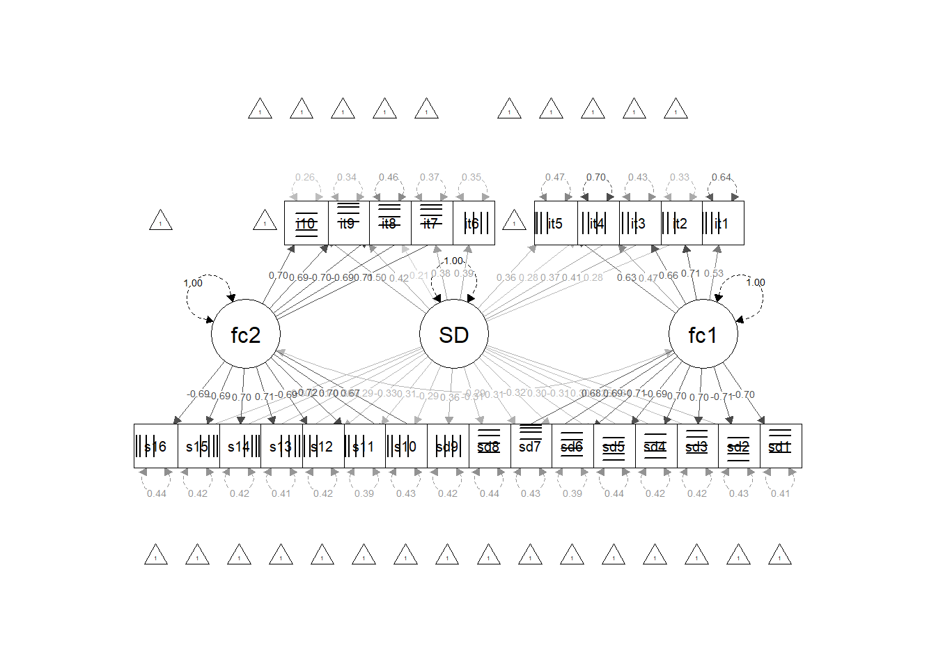
For large models, path diagrams can become visually dense. They are most useful for checking the intended parameterization rather than replacing numerical inspection of the fitted model.
10 Choosing a Strategy
No social-desirability control is assumption-free. A useful choice depends on what information the study design can provide.
| Situation | Particularly relevant strategy |
|---|---|
| Existing dataset with a separate SD scale | Sensitivity analyses; factor-based control if marker assumptions are plausible |
| Hypothesis that only some respondents fake | Factor-mixture model |
| Experimental manipulation of response context | Common-method-factor / repeated-measures design |
| New instrument under development | Peabody-style balanced content or related item-design strategies |
| Desire to extend an identified evaluative factor to ordinary items | MIMIC-quadruplet model |
A response-bias adjustment is useful only when the model separates nuisance variance from substantive variance credibly. A poorly identified desirability factor can remove meaningful construct variance and produce scores that appear cleaner while being less valid.
11 Concluding Remarks
Social desirability is not a single statistical nuisance with a universal correction. It can reflect intentional self-presentation, self-favoring beliefs, socially valued substantive traits, item evaluation, or shared method variance. Different control procedures target different parts of that problem.
The practical lesson is therefore to make the assumed response process explicit. If social desirability is represented as a latent method factor, the researcher should explain why the factor is identifiable and why it is distinguishable from substantive content. If it is addressed through item design, the evaluative and descriptive manipulations should be defensible. If a separate desirability scale is used, its score should not be treated automatically as a pure measure of dishonesty.
The next chapter turns to another response tendency—acquiescence—and shows why simply reversing item wording is not always sufficient to remove it.
8.4 Social Desirability as Systematic Score Variance
In Classical Test Theory, an observed score is commonly written as
\[ X = T + E, \]
where \(T\) is the expected score across hypothetical replications of the same measurement procedure and \(E\) is random error.
A key implication is that a stable response distortion produced by a motivating context is not well represented as random error. A more useful conceptual decomposition is
\[ X_{\text{motivated}} = T_{\text{target}} + S_{\text{response}} + E, \]
where \(S_{\text{response}}\) represents one or more systematic influences associated with the response situation. These influences can include dispositional, attitudinal, and situational components (Ziegler et al., 2011).
At the variance level,
\[ \operatorname{Var}(X) = \operatorname{Var}(T_{\text{target}}) + \operatorname{Var}(S_{\text{response}}) + 2\operatorname{Cov}(T_{\text{target}},S_{\text{response}}) + \operatorname{Var}(E). \]
This form makes an important point explicit: the response-related component can be systematic and can covary with substantive trait variance. Consequently, controlling social desirability is not as simple as subtracting a nuisance score that is guaranteed to be independent of the construct.