7 Exploratory Graph Analysis
Psychological and educational instruments often contain many items, but the substantive interpretation usually concerns a smaller number of dimensions. A central psychometric question is therefore:
How many dimensions are represented by the observed item responses, and which items belong to each dimension?
Factor-analytic approaches traditionally address this question using factor-retention procedures such as the Kaiser–Guttman criterion, parallel analysis, and related methods. These procedures can work well, but none is universally accurate. The eigenvalue-greater-than-one rule, for example, can both under- and overestimate dimensionality (Zwick & Velicer, 1986), while the performance of parallel analysis can depend on features such as response format and the particular procedure used (Green et al., 2016).
Exploratory Graph Analysis (EGA) was proposed as an alternative network-based approach to dimensionality estimation (H. F. Golino & Epskamp, 2017). Rather than beginning with an eigenvalue-retention rule, EGA estimates a network among the observed variables and then uses community detection to identify groups of strongly connected items.
This chapter develops EGA through three main stages:
- Unique Variable Analysis (UVA): identify potentially redundant or locally dependent items.
- Exploratory Graph Analysis: estimate the item network and identify communities.
- Bootstrap EGA: evaluate how consistently the dimensions and item assignments are recovered across resampled datasets.
The final section implements the complete workflow in R using EGAnet.
7.1 What Is Exploratory Graph Analysis?
Network psychometrics represents variables as nodes and statistical relationships among them as edges. In an EGA of questionnaire items, each item becomes a node, and the estimated association between two items is represented by the edge connecting them.
EGA then applies a community-detection algorithm to this network. Groups of items that are more strongly connected with one another than with other parts of the network are identified as communities, which are interpreted as candidate dimensions (H. Golino et al., 2020; H. F. Golino & Epskamp, 2017).
| In EFA | In EGA |
|---|---|
| Observed item | Node |
| Factor loading | Network loading / item-community association |
| Latent dimension | Detected network community |
| Factor-retention method | Community-detection procedure |
| Stability of loading structure | Bootstrap item and dimension stability |
7.1.1 Relationship to factor models
EGA does not require us to assume that psychological variables are literally generated by direct interactions among observed items. If data are generated by a reflective common-factor model, items influenced by the same factor can also form communities in a network (H. F. Golino & Epskamp, 2017). Simulation research has shown that EGA can recover factor dimensionality with accuracy comparable to strong traditional factor-retention procedures across many conditions (H. Golino et al., 2020).
EGA estimates statistical communities. Giving those communities psychological meaning still requires item content, theory, and validity evidence. Finding five communities does not, by itself, prove that five psychological traits exist.
7.2 The EGA Workflow
A useful way to think about the procedure is:
| Stage | Main question | Typical function |
|---|---|---|
| 1. UVA | Are some items redundant beyond the broader dimensional structure? | UVA() |
| 2. EGA | How many communities are present, and which items belong to each? | EGA() |
| 3. Bootstrap EGA | Is this dimensional solution stable across replicated samples? | bootEGA() |
| 4. Stability diagnostics | Which dimensions and items are recovered consistently? |
dimensionStability() / itemStability()
|
8 1. Unique Variable Analysis
8.1 Local Independence and Redundancy
In a reflective latent-variable model, indicators are expected to become independent after conditioning on the relevant latent variable. This property is called local independence.
When two indicators remain strongly related beyond what is expected from the broader structure, they may contain redundant content or additional shared dependence. Such local dependence can distort estimates of internal structure and other psychometric quantities (Christensen et al., 2023).
Unique Variable Analysis (UVA) was developed to detect these potentially redundant pairs using network psychometric methods (Christensen et al., 2023). One of its central quantities is weighted topological overlap (wTO), which considers both the direct relation between two nodes and the similarity of their connections with the rest of the network (Nowick et al., 2009).
A commonly presented weighted topological overlap measure is
\[ \omega_{ij} = \frac{ \sum_{u} a_{iu}a_{uj}+a_{ij} }{ \min(k_i,k_j)+1-a_{ij} }, \]
where:
- \(a_{ij}\) is the edge weight between nodes \(i\) and \(j\);
- \(u\) indexes connections shared by nodes \(i\) and \(j\); and
- \(k_i\) and \(k_j\) summarize the strength of the connections of the two nodes.
Higher values indicate that two variables occupy very similar positions in the network and may contain overlapping information.
In the UVA framework proposed by Christensen et al. (2023), cutoff-based procedures performed better overall than significance-based approaches. A value around .25 is commonly used as a practical indication of potentially important redundancy.
Two items can be statistically redundant while still serving different substantive purposes. Before removing an item, inspect its wording, construct coverage, response format, and role in the measure.
8.1.1 How UVA reduces redundant sets
When automatic reduction is requested, UVA must decide which variable to retain from a redundant set. The logic differs according to the number of variables involved:
| Redundant set | General logic |
|---|---|
| Duplet | Retain the variable that is less redundant with the remainder of the item set |
| Triplet or larger set | Retain the variable that best represents the redundant group and remove the others |
The objective is not simply to remove correlated items. It is to reduce local redundancy before estimating dimensionality.
9 2. Exploratory Graph Analysis
EGA combines two operations:
- estimate a network describing conditional relationships among the variables; and
- apply a community-detection algorithm to identify clusters of nodes.
The original EGA implementation used an EBIC graphical lasso network followed by Walktrap community detection (H. F. Golino & Epskamp, 2017).
9.1 Partial Correlations
A zero-order correlation between two variables contains both their direct association and associations that may be explained through other variables. In contrast, a partial correlation describes the association between two variables after statistically controlling for the remaining variables in the model.
For a covariance matrix
\[ \Sigma, \]
define the precision matrix
\[ K = \Sigma^{-1}. \]
The partial correlation between variables \(i\) and \(j\), controlling for all remaining variables, is
\[ \rho_{ij\cdot -ij} = -\frac{k_{ij}} {\sqrt{k_{ii}k_{jj}}}. \]
Thus, the inverse covariance matrix provides the information needed to construct the full-order partial-correlation network (H. Golino et al., 2020).
If two items are correlated only because both are related to several other items, their partial correlation may be small. This helps the network emphasize more specific conditional relationships.
9.2 EBICglasso
Estimating every possible partial correlation can produce a dense network containing many weak or unstable edges. The graphical lasso addresses this by applying an \(L_1\) penalty to elements of the precision matrix, shrinking some estimates exactly to zero (Friedman et al., 2008).
The tuning parameter
\[ \lambda \]
controls the degree of regularization:
| \(\lambda\) | Consequence |
|---|---|
| Smaller | More edges remain; the network is denser |
| Larger | More estimates are shrunk to zero; the network is sparser |
The EGA approach historically fits networks across candidate values of \(\lambda\) and selects a model using the Extended Bayesian Information Criterion (EBIC). EBIC extends BIC by adding a penalty that is useful when the candidate model space is large (Chen & Chen, 2008).
A second tuning quantity,
\[ \gamma, \]
controls how strongly EBIC favors sparse models. Larger values of \(\gamma\) produce a stronger preference for simpler networks; when \(\gamma=0\), the additional EBIC penalty disappears and the criterion reduces to the ordinary BIC form (Chen & Chen, 2008).
Do not confuse \(\lambda\) and \(\gamma\).
- \(\lambda\) controls the amount of shrinkage used to estimate a particular graphical-lasso network.
- \(\gamma\) changes the EBIC penalty used when selecting among candidate networks.
9.3 Community Detection: Walktrap
After estimating the network, EGA uses a community-detection algorithm to partition the nodes.
The original EGA implementation used Walktrap, an algorithm based on short random walks (Pons & Latapy, 2006). The intuition is that a short random walk tends to remain within a densely connected community because there are many strong paths among nodes belonging to the same cluster.
A simplified view of the process is:
- construct transition probabilities from the weighted network;
- perform short random walks;
- use similarities in the random-walk behavior to progressively combine nodes and communities; and
- select a partition using the community structure of the graph (Newman, 2006; Pons & Latapy, 2006).
Each resulting community is interpreted as a candidate psychometric dimension.
Modern versions of EGAnet provide several network estimators and community-detection algorithms. In the R tutorial below, we explicitly request model = "glasso" and algorithm = "walktrap" so that the code matches the EBICglasso + Walktrap approach explained in this chapter (H. Golino & Christensen, 2026).
10 3. Stability of the EGA Solution
A single estimated structure may reflect sampling variation. Bootstrap EGA therefore repeatedly estimates EGA solutions from replicated datasets and examines how consistently the dimensional structure is recovered (Christensen & Golino, 2021).
bootEGA() can use either a parametric procedure based on the empirical association structure or nonparametric resampling of the observed cases. Across replications, the procedure records:
- the number of dimensions detected;
- community membership of each item;
- the estimated networks; and
- stability information about dimensions and items.
The bootstrap can also be used to obtain a typical network structure based on median pairwise relationships across bootstrap samples (Christensen & Golino, 2021).
10.1 Structural Consistency
Structural consistency describes how often an empirically identified dimension is reproduced with the same item composition across bootstrap samples.
If a dimension has low structural consistency, the exact composition of that dimension is changing substantially across replications.
10.2 Item Stability
Item stability describes how often an individual item returns to the same empirical dimension across bootstrap replications.
An item with low stability may:
- move between neighboring dimensions;
- occupy a boundary between communities;
- contain content associated with multiple constructs; or
- reflect an unstable dimensional solution.
Values around .70 to .75 have commonly been used as practical reference points in EGA applications (Christensen & Golino, 2021), but these values should be treated as descriptive guidance rather than universal psychometric laws.
A solution can repeatedly produce the same number of dimensions while individual items move between them. For this reason, stability should not be evaluated only from the bootstrap distribution of the number of communities.
11 Running EGA Step by Step in R
The tutorial uses EGAnet (H. Golino & Christensen, 2026), the bfi personality data and item dictionary available through the psych/psychTools ecosystem (Revelle, 2023), and lavaan for an optional CFA follow-up (Rosseel, 2012).
11.1 Install the Packages
Installation only needs to be performed once.
Load the packages:
[1;m[4;m
EGAnet (version 2.4.1)[0m[0m

For help getting started, see <https://r-ega.net>

For bugs and errors, submit an issue to <https://github.com/hfgolino/EGAnet/issues>
Anexando pacote: 'psych'O seguinte objeto é mascarado por 'package:EGAnet':
CFAThis is lavaan 0.7-2
lavaan is FREE software! Please report any bugs.
Anexando pacote: 'lavaan'O seguinte objeto é mascarado por 'package:psych':
cor2cov11.2 Prepare the BFI Items
The example uses the first 25 variables from the bfi dataset, which represent personality items from the Big Five item set.
For readability in UVA output, we will also use the corresponding item descriptions from the psychTools dictionary.
11.3 Step 1: Run Unique Variable Analysis
Variable pairs with wTO > 0.30 (large-to-very large redundancy)

            node_i                node_j   wto
 Get angry easily. Get irritated easily. 0.431

----

Variable pairs with wTO > 0.25 (moderate-to-large redundancy)

----

Variable pairs with wTO > 0.20 (small-to-moderate redundancy)

                                    node_i
                         Don't talk a lot.
                   Am exacting in my work.
 Am indifferent to the feelings of others.
           Do things in a half-way manner.
               Know how to comfort others.
                         Get angry easily.
                Have frequent mood swings.
         Inquire about others' well-being.
                                node_j   wto
 Find it difficult to approach others. 0.226
 Continue until everything is perfect. 0.225
     Inquire about others' well-being. 0.219
                        Waste my time. 0.209
             Make people feel at ease. 0.207
            Have frequent mood swings. 0.205
                      Often feel blue. 0.204
           Know how to comfort others. 0.203
The output identifies pairs or sets of items with potentially important topological overlap and reports the reduction suggested by UVA.
The retained and removed variables can be inspected with:
In this example, the interpretation should focus on the content of the flagged items as well as the wTO value. Similar wording such as “getting angry easily” and “getting irritated easily” provides a substantive reason why two variables might behave redundantly.
The reduced dataset is available directly from the UVA object:
Do not let UVA() silently decide the final questionnaire. Treat the automatic reduction as a statistical recommendation and document the substantive reason for retaining or removing each flagged item.
11.4 Step 2: Estimate the EGA Structure
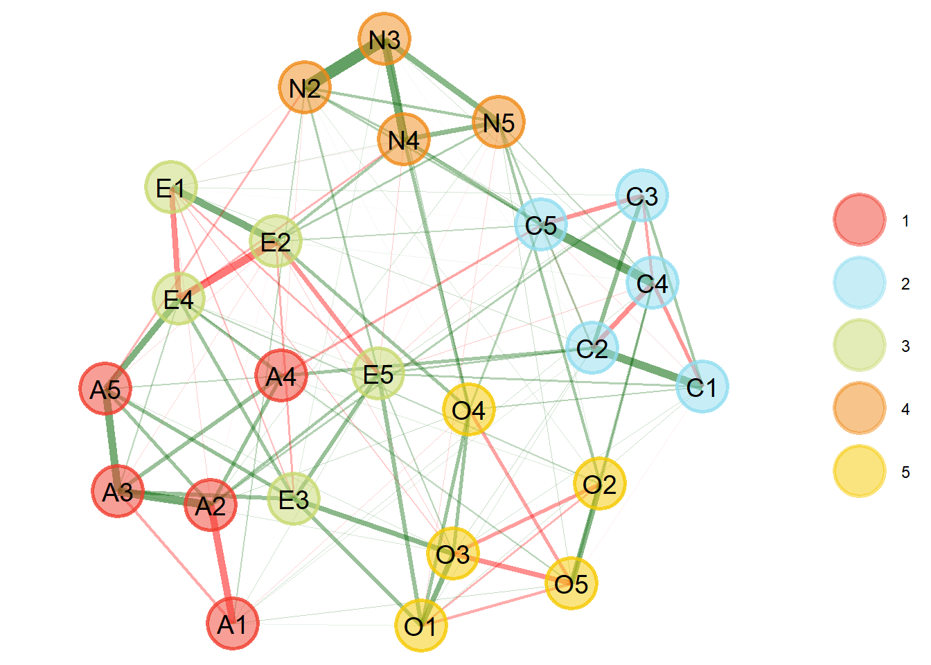
To match the method explained earlier in the chapter, we explicitly request a graphical-lasso network and Walktrap community detection.
Model: GLASSO (EBIC with gamma = 0.5)
Correlations: auto
Lambda: 0.0597096451199323 (n = 100, ratio = 0.1)

Number of nodes: 24
Number of edges: 125
Edge density: 0.453

Non-zero edge weights:
     M    SD    Min   Max
 0.041 0.112 -0.270 0.396

----

Algorithm:  Walktrap

Number of communities:  5

A1 A2 A3 A4 A5 C1 C2 C3 C4 C5 E1 E2 E3 E4 E5 N2 N3 N4 N5 O1 O2 O3 O4 O5
 1  1  1  1  1  2  2  2  2  2  3  3  3  3  3  4  4  4  4  5  5  5  5  5

----

Unidimensional Method: Louvain
Unidimensional: No

----

TEFI: -24.989
The EGA plot uses color to distinguish detected communities. Each node is an item, and each community represents a candidate dimension.
A text summary is available with:
Model: GLASSO (EBIC with gamma = 0.5)
Correlations: auto
Lambda: 0.0597096451199323 (n = 100, ratio = 0.1)

Number of nodes: 24
Number of edges: 125
Edge density: 0.453

Non-zero edge weights:
     M    SD    Min   Max
 0.041 0.112 -0.270 0.396

----

Algorithm:  Walktrap

Number of communities:  5

A1 A2 A3 A4 A5 C1 C2 C3 C4 C5 E1 E2 E3 E4 E5 N2 N3 N4 N5 O1 O2 O3 O4 O5
 1  1  1  1  1  2  2  2  2  2  3  3  3  3  3  4  4  4  4  5  5  5  5  5

----

Unidimensional Method: Louvain
Unidimensional: No

----

TEFI: -24.989
The summary provides several layers of information:
| Output | Interpretation |
|---|---|
| Network model | How the item network was estimated |
| Network characteristics | Number of nodes, edges, edge density, and edge summaries |
| Community algorithm | How communities were identified |
| Number of communities | Estimated dimensionality |
| Item membership | Which community each item belongs to |
| Unidimensionality information | Whether a one-dimensional solution should be considered |
| TEFI, when available | Entropy-based information that can help compare dimensional structures |
The Total Entropy Fit Index (TEFI) was proposed as an information- theoretic approach for comparing dimensional structures (H. Golino et al., 2021). Like other model-comparison quantities, it should be interpreted comparatively rather than as an isolated pass/fail number.
If EGA detects five communities in the BFI data, the result is statistically consistent with the familiar five-dimensional organization of Big Five personality items. The EGA result does not prove the Big Five theory; it shows that the observed network contains a five-community structure that can be interpreted in relation to that theory.
11.5 Step 3: Bootstrap the EGA
Bootstrap EGA is the most computationally intensive part of this chapter. The example uses 500 bootstrap replications, matching a common choice in the EGA literature (Christensen & Golino, 2021).
Show bootstrap EGA code
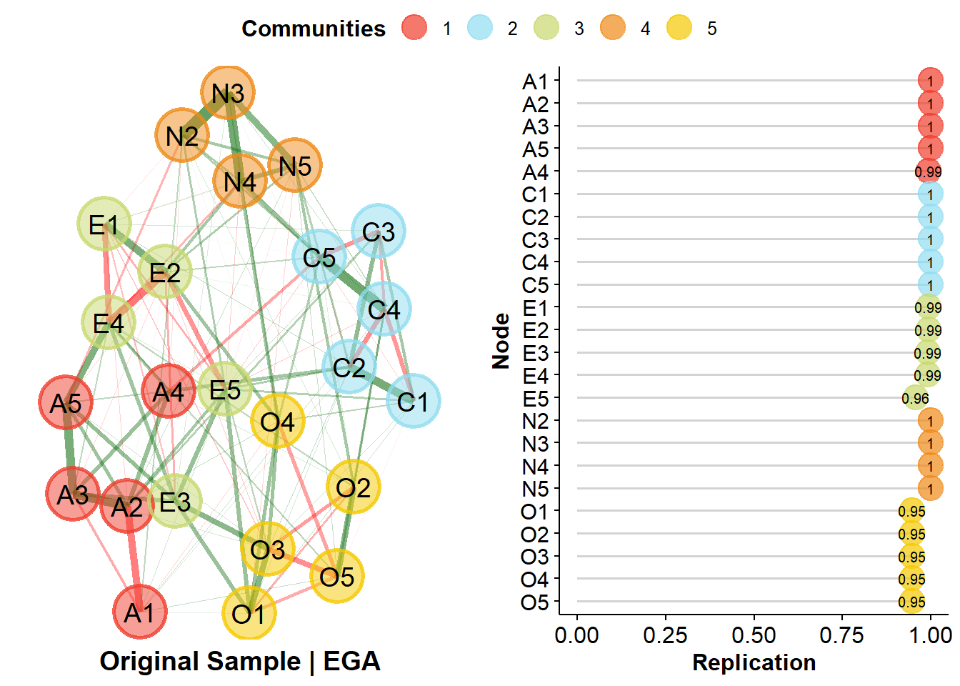
The cache option is intentional: once the bootstrap has been computed, Quarto can reuse the stored result rather than recomputing 500 EGA solutions every time the chapter is rendered.
Inspect the bootstrap summary with:
Model: GLASSO (EBIC)
Correlations: auto
Algorithm:  Walktrap
Unidimensional Method:  Louvain

----

EGA Type: EGA
Bootstrap Samples: 500 (Parametric)

                4     5
Frequency:  0.058 0.942

Median dimensions: 5 [4.54, 5.46] 95% CI
Important results include:
- how often each number of communities was recovered;
- the median number of communities;
- uncertainty in the number of dimensions; and
- information about the estimation procedure used across replications.
A bootstrap distribution concentrated around the empirical number of dimensions is reassuring, but it is not sufficient by itself. We should also inspect the stability of the dimensions and the items.
11.6 Dimension and Item Stability
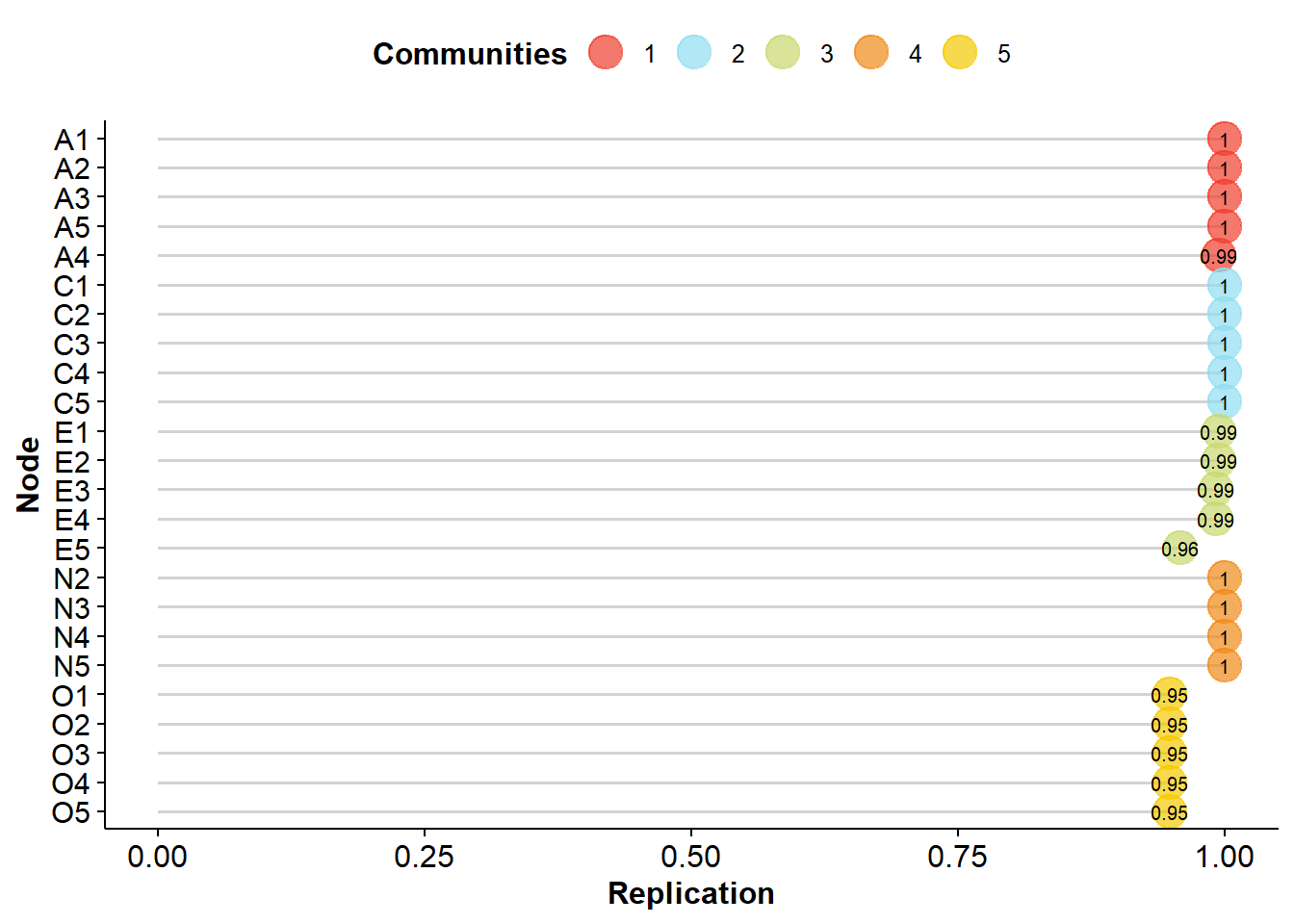
EGA Type: EGA
Bootstrap Samples: 500 (Parametric)

Proportion Replicated in Dimensions:

   A1    A2    A3    A4    A5    C1    C2    C3    C4    C5    E1    E2    E3
1.000 1.000 1.000 0.994 1.000 1.000 1.000 1.000 1.000 1.000 0.994 0.994 0.992
   E4    E5    N2    N3    N4    N5    O1    O2    O3    O4    O5
0.992 0.958 1.000 1.000 1.000 1.000 0.948 0.948 0.948 0.948 0.948

----

Structural Consistency:

    1     2     3     4     5
0.994 1.000 0.966 1.000 0.948
The resulting diagnostics show how consistently the empirical dimensions and their items are recovered across bootstrap samples.
Interpret stability at two levels:
- Dimension-level stability: Is the same set of items repeatedly recovered as a dimension?
- Item-level stability: Does each item repeatedly return to its original empirical dimension?
An item that repeatedly switches between dimensions deserves particular attention, even if the total number of dimensions remains stable.
Low item stability is not automatically a reason for deletion. It may indicate ambiguous wording, construct overlap, a boundary item, local dependence, or a genuinely complex psychological structure.
11.7 Network Loadings
Network loadings provide information analogous in purpose—not identical in mathematics—to factor loadings. They quantify how strongly variables are connected with their own and other network dimensions (Christensen et al., 2020).
The default 'loading.method' has changed to "revised" in {EGAnet} version >= 2.0.7.

For the previous default (version <= 2.0.6), use `loading.method = "original"`Loading Method: Revised
1 2 3 4 5
A2 0.585 0.04 0.078 0.017 0.026
A3 0.579 0 0.124 0 0.013
A5 0.33 0 0.239 -0.038 0.015
A4 0.248 0.12 0.062 -0.007 -0.015
A1 -0.253 -0.009 0.014 0.03 -0.035
C2 0.057 0.465 0.021 0.039 0.037
C1 0 0.395 0.041 0 0.075
C3 0.042 0.379 0.013 0 0
C5 -0.061 -0.378 -0.051 0.118 0.035
C4 -0.019 -0.519 -0.024 0.068 -0.1
E4 0.228 0 0.441 -0.041 -0.061
E3 0.173 0 0.29 0.008 0.2
E5 0.049 0.147 0.289 0.025 0.117
E1 -0.014 0.033 -0.421 0.006 -0.029
E2 -0.025 -0.03 -0.559 0.104 0.055
N3 0 -0.017 0.008 0.671 0.028
N2 -0.078 -0.043 0.055 0.437 -0.01
N4 0 -0.098 -0.135 0.412 0.071
N5 0.018 0.011 -0.052 0.349 -0.1
O3 0.027 0.039 0.191 0 0.485
O1 -0.004 0.028 0.161 -0.012 0.376
O4 0.039 -0.004 -0.072 0.091 0.274
O2 0.01 -0.054 0.03 0.07 -0.322
O5 -0.02 -0.046 0.029 0.02 -0.456
Standardized loadings >= |0.00| are displayed. To change this 'minimum', use `print(net.loads_object, minimum = 0.10)`When interpreting network loadings, examine:
- which dimension has the largest loading for each item;
- whether an item has meaningful loadings on multiple dimensions; and
- whether the loading pattern agrees with the detected community membership.
As with factor loadings, item content should guide the substantive interpretation.
11.8 Optional Follow-Up: CFA of the EGA Structure
EGA is exploratory. If the detected structure is theoretically meaningful, one possible follow-up is to translate that structure into a confirmatory factor model.
EGAnet provides a convenience function for this purpose:
[1] "A1" "A2" "A3" "A4" "A5"
[1] "C1" "C2" "C3" "C4" "C5"
[1] "E1" "E2" "E3" "E4" "E5"
[1] "N2" "N3" "N4" "N5"
[1] "O1" "O2" "O3" "O4" "O5"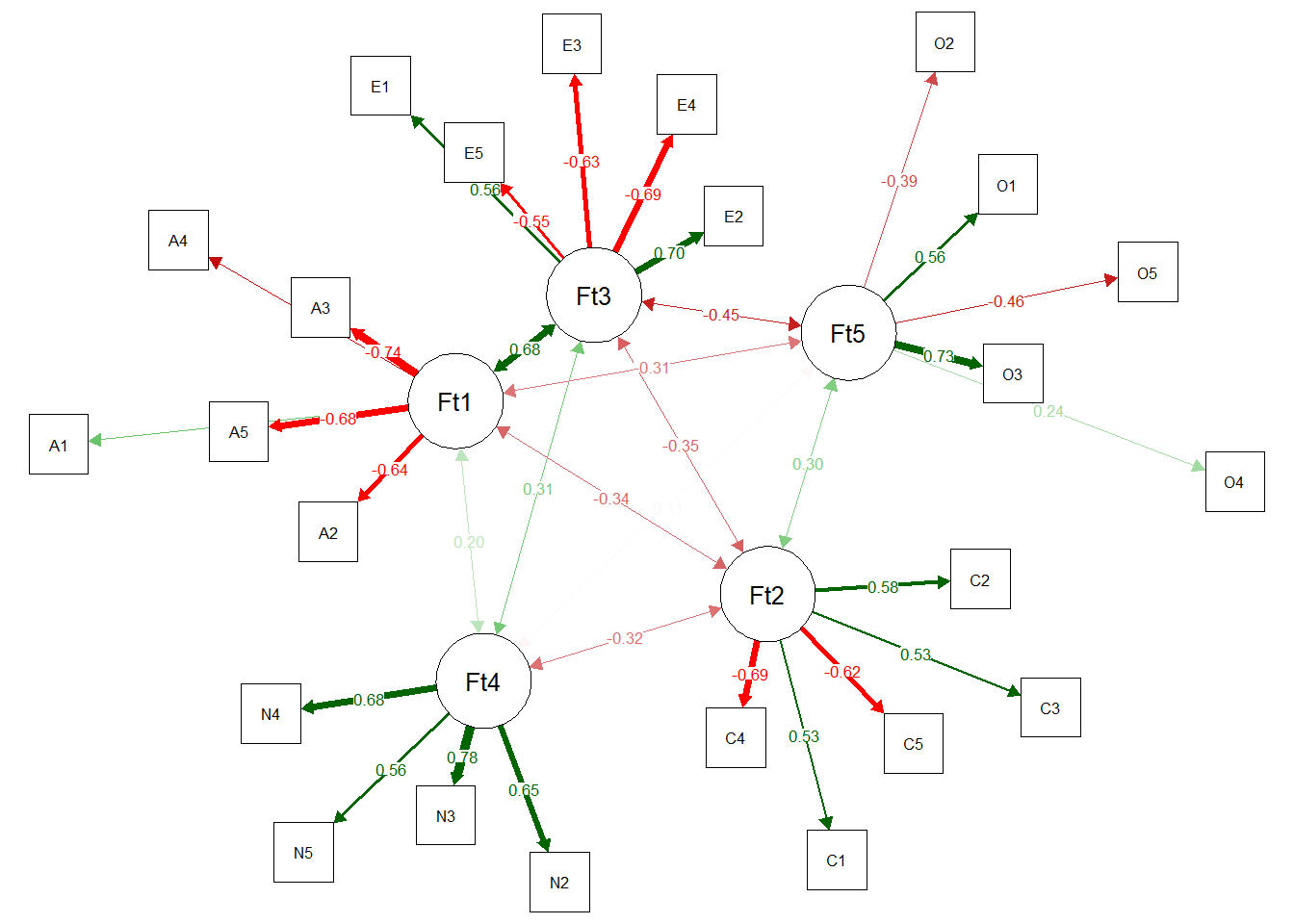
Fit measures can then be extracted from the underlying lavaan model:
                         npar                          fmin
                       82.000                         0.738
                        chisq                            df
                     4132.221                       242.000
                       pvalue                  chisq.scaled
                        0.000                      3570.714
                    df.scaled                 pvalue.scaled
                      242.000                         0.000
         chisq.scaling.factor                baseline.chisq
                        1.157                     17655.215
                  baseline.df               baseline.pvalue
                      276.000                         0.000
        baseline.chisq.scaled            baseline.df.scaled
                    14781.836                       276.000
       baseline.pvalue.scaled baseline.chisq.scaling.factor
                        0.000                         1.194
                          cfi                           tli
                        0.776                         0.745
                   cfi.scaled                    tli.scaled
                        0.771                         0.738
                   cfi.robust                    tli.robust
                        0.777                         0.746
                         nnfi                           rfi
                        0.745                         0.733
                          nfi                          pnfi
                        0.766                         0.672
                          ifi                           rni
                        0.777                         0.776
                  nnfi.scaled                    rfi.scaled
                        0.738                         0.725
                   nfi.scaled                   pnfi.scaled
                        0.758                         0.665
                   ifi.scaled                    rni.scaled
                        0.771                         0.771
                  nnfi.robust                    rni.robust
                        0.746                         0.777
                         logl             unrestricted.logl
                  -109988.969                   -107922.858
                          aic                           bic
                   220141.938                    220628.802
                       ntotal                          bic2
                     2800.000                    220368.260
            scaling.factor.h1             scaling.factor.h0
                        1.155                         1.147
                        rmsea                rmsea.ci.lower
                        0.076                         0.074
               rmsea.ci.upper                rmsea.ci.level
                        0.078                         0.900
                 rmsea.pvalue                rmsea.close.h0
                        0.000                         0.050
        rmsea.notclose.pvalue             rmsea.notclose.h0
                        0.000                         0.080
                 rmsea.scaled         rmsea.ci.lower.scaled
                        0.070                         0.068
        rmsea.ci.upper.scaled           rmsea.pvalue.scaled
                        0.072                         0.000
 rmsea.notclose.pvalue.scaled                  rmsea.robust
                        0.000                         0.076
        rmsea.ci.lower.robust         rmsea.ci.upper.robust
                        0.074                         0.078
          rmsea.pvalue.robust  rmsea.notclose.pvalue.robust
                        0.000                         0.001
                          rmr                    rmr_nomean
                        0.144                         0.150
                         srmr                  srmr_bentler
                        0.070                         0.070
          srmr_bentler_nomean                          crmr
                        0.073                         0.073
                  crmr_nomean                    srmr_mplus
                        0.076                         0.070
            srmr_mplus_nomean                           gfi
                        0.073                         0.896
                 gfi.ci.lower                  gfi.ci.upper
                        0.891                         0.901
                 gfi.ci.level                    gfi.robust
                        0.900                         0.896
          gfi.ci.lower.robust           gfi.ci.upper.robust
                        0.891                         0.901
                        cn_05                         cn_01
                      190.246                       201.638
                   gfi_lisrel                   agfi_lisrel
                        0.992                         0.990
                         pgfi                           mfi
                        0.741                         0.499
                         ecvi
                        1.534
attr(,"scaled.test")
[1] "yuan.bentler.mplus"If the same dataset is used to discover the EGA structure and then fit a CFA, the CFA is not an independent confirmation of that structure. A stronger design estimates the exploratory structure in one sample and evaluates it in another sample or an external dataset.
12 A Compact EGA Interpretation Guide
| Result | Ask… |
|---|---|
| UVA | Are any items locally redundant, and does their content explain why? |
| EGA communities | How many dimensions are identified, and do the grouped items make substantive sense? |
| Edges | Which conditional item relationships remain after network estimation? |
| Network loadings | Which community is each item most strongly associated with? |
| Bootstrap dimensionality | Is the same number of communities recovered consistently? |
| Structural consistency | Is each empirical dimension recovered with the same composition? |
| Item stability | Do individual items remain in the same community? |
| TEFI / model comparison | Does one candidate dimensional structure receive better comparative support? |
| CFA follow-up | Does a theoretically specified version of the exploratory solution reproduce the data reasonably well? |
13 How to Report an EGA
A transparent report should describe enough of the procedure for another researcher to reproduce the dimensionality decision. At minimum, report:
- the variables included in the analysis;
- whether and how UVA was used;
- the network estimation method;
- the community-detection algorithm;
- the estimated number of communities;
- the item membership of each community;
- the bootstrap type and number of replications;
- the distribution of recovered dimensionality;
- dimension and item stability;
- any network-loading or entropy-fit information used in interpretation; and
- any item reductions or modifications made after inspecting the results.
For the BFI tutorial, the analytic description could follow this form:
Exploratory Graph Analysis was conducted on the 25 BFI personality items. Unique Variable Analysis was first used to identify potentially redundant variables. EGA was then estimated using a graphical-lasso network and Walktrap community detection. The stability of the dimensional structure was evaluated using 500 bootstrap replications. The number and composition of the detected communities, structural consistency, item stability, and network loadings were considered jointly when interpreting the solution.
Insert the actual numerical results from the fitted models when reporting an empirical analysis.
14 Concluding Remarks
EGA provides a complementary approach to dimensionality estimation. Its main advantage is that it returns both an estimate of the number of dimensions and an explicit representation of which items belong to those dimensions. UVA and bootstrap EGA extend this workflow by making local redundancy and structural stability part of the analysis rather than afterthoughts.
At the same time, EGA does not remove the need for psychometric theory. The community-detection algorithm identifies statistical structure; the researcher still has to decide whether the communities form coherent constructs, whether item redundancy is substantively problematic, and whether the solution is stable enough to support further interpretation.
The most useful reading of EGA is therefore not simply “the algorithm found five dimensions.” A stronger conclusion asks whether the number of dimensions, item memberships, network loadings, bootstrap stability, and theoretical interpretation all converge on the same measurement structure.